Ansible module for Dell EMC Isilon has been released 2 months before and I’ve seen many people are interested in it. Here is a quick demo of how to use it to create and mount an NFS export. For further details, please go to our github community: https://github.com/dell/ansible-isilon
OneFS Endurant Cache
The earlier blog post on multi-threaded I/O generated several questions on synchronous writes in OneFS. So this seemed like a useful topic to explore in a bit more detail.
OneFS natively provides a caching mechanism for synchronous writes – or writes that require a stable write acknowledgement to be returned to a client. This functionality is known as the Endurant Cache, or EC.
The EC operates in conjunction with the OneFS write cache, or coalescer, to ingest, protect and aggregate small, synchronous NFS writes. The incoming write blocks are staged to NVRAM, ensuring the integrity of the write, even during the unlikely event of a node’s power loss. Furthermore, EC also creates multiple mirrored copies of the data, further guaranteeing protection from single node and, if desired, multiple node failures.
EC improves the latency associated with synchronous writes by reducing the time to acknowledgement back to the client. This process removes the Read-Modify-Write (R-M-W) operations from the acknowledgement latency path, while also leveraging the coalescer to optimize writes to disk. EC is also tightly coupled with OneFS’ multi-threaded I/O (Multi-writer) process, to support concurrent writes from multiple client writer threads to the same file. And the design of EC ensures that the cached writes do not impact snapshot performance.
The endurant cache uses write logging to combine and protect small writes at random offsets into 8KB linear writes. To achieve this, the writes go to special mirrored files, or ‘Logstores’. The response to a stable write request can be sent once the data is committed to the logstore. Logstores can be written to by several threads from the same node, and are highly optimized to enable low-latency concurrent writes.
Note that if a write uses the EC, the coalescer must also be used. If the coalescer is disabled on a file, but EC is enabled, the coalescer will still be active with all data backed by the EC.
So what exactly does an endurant cache write sequence look like?
Say an NFS client wishes to write a file to an Isilon cluster over NFS with the O_SYNC flag set, requiring a confirmed or synchronous write acknowledgement. Here is the sequence of events that occur to facilitate a stable write.
1) A client, connected to node 3, begins the write process sending protocol level blocks. 4K is the optimal block size for the endurant cache.
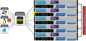
2) The NFS client’s writes are temporarily stored in the write coalescer portion of node 3’s RAM. The Write Coalescer aggregates uncommitted blocks so that the OneFS can, ideally, write out full protection groups where possible, reducing latency over protocols that allow “unstable” writes. Writing to RAM has far less latency that writing directly to disk.
3) Once in the write coalescer, the endurant cache log-writer process writes mirrored copies of the data blocks in parallel to the EC Log Files.
The protection level of the mirrored EC log files is the same as that of the data being written by the NFS client.
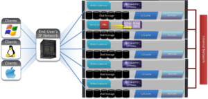
4) When the data copies are received into the EC Log Files, a stable write exists and a write acknowledgement (ACK) is returned to the NFS client confirming the stable write has occurred. The client assumes the write is completed and can close the write session.
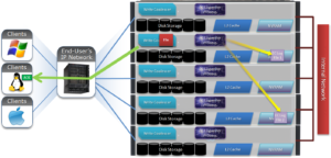
5) The write coalescer then processes the file just like a non-EC write at this point. The write coalescer fills and is routinely flushed as required as an asynchronous write via to the block allocation manager (BAM) and the BAM safe write (BSW) path processes.
6) The file is split into 128K data stripe units (DSUs), parity protection (FEC) is calculated and FEC stripe units (FSUs) are created.
7) The layout and write plan is then determined, and the stripe units are written to their corresponding nodes’ L2 Cache and NVRAM. The EC logfiles are cleared from NVRAM at this point. OneFS uses a Fast Invalid Path process to de-allocate the EC Log Files from NVRAM.
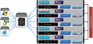
8) Stripe Units are then flushed to physical disk.
9) Once written to physical disk, the data stripe Unit (DSU) and FEC stripe unit (FSU) copies created during the write are cleared from NVRAM but remain in L2 cache until flushed to make room for more recently accessed data.
As far as protection goes, the number of logfile mirrors created by EC is always one more than the on-disk protection level of the file. For example:
| File Protection Level | Number of EC Mirrored Copies |
| +1n | 2 |
| 2x | 3 |
| +2n | 3 |
| +2d:1n | 3 |
| +3n | 4 |
| +3d:1n | 4 |
| +4n | 5 |
The EC mirrors are only used if the initiator node is lost. In the unlikely event that this occurs, the participant nodes replay their EC journals and complete the writes.
If the write is an EC candidate, the data remains in the coalescer, an EC write is constructed, and the appropriate coalescer region is marked as EC. The EC write is a write into a logstore (hidden mirrored file) and the data is placed into the journal.
Assuming the journal is sufficiently empty, the write is held there (cached) and only flushed to disk when the journal is full, thereby saving additional disk activity.
An optimal workload for EC involves small-block synchronous, sequential writes – something like an audit or redo log, for example. In that case, the coalescer will accumulate a full protection group’s worth of data and be able to perform an efficient FEC write.
The happy medium is a synchronous small block type load, particularly where the I/O rate is low and the client is latency-sensitive. In this case, the latency will be reduced and, if the I/O rate is low enough, it won’t create serious pressure.
The undesirable scenario is when the cluster is already spindle-bound and the workload is such that it generates a lot of journal pressure. In this case, EC is just going to aggravate things.
So how exactly do you configure the endurant cache?
Although on by default, setting the efs.bam.ec.mode sysctl to value ‘1’ will enable the Endurant Cache:
# isi_sysctl_cluster efs.bam.ec.mode=1
EC can also be enabled & disabled per directory:
# isi set -c [on|off|endurant_all|coal_only] <directory_name>
To enable the coalescer but switch of EC, run:
# isi set -c coal_only
And to disable the endurant cache completely:
# isi_for_array –s isi_sysctl_cluster efs.bam.ec.mode=0
A return value of zero on each node from the following command will verify that EC is disabled across the cluster:
# isi_for_array –s sysctl efs.bam.ec.stats.write_blocks efs.bam.ec.stats.write_blocks: 0
If the output to this command is incrementing, EC is delivering stable writes.
Be aware that if the Endurant Cache is disabled on a cluster the sysctl efs.bam.ec.stats.write_blocks output on each node will not return to zero, since this sysctl is a counter, not a rate. These counters won’t reset until the node is rebooted.
As mentioned previously, EC applies to stable writes. Namely:
- Writes with O_SYNC and/or O_DIRECT flags set
- Files on synchronous NFS mounts
When it comes to analyzing any performance issues involving EC workloads, consider the following:
- What changed with the workload?
- If upgrading OneFS, did the prior version also have EC enable?
- If the workload has moved to new cluster hardware:
- Does the performance issue occur during periods of high CPU utilization?
- Which part of the workload is creating a deluge of stable writes?
- Was there a large change in spindle or node count?
- Has the OneFS protection level changed?
- Is the SSD strategy the same?
Disabling EC is typically done cluster-wide and this can adversely impact certain workflow elements. If the EC load is localized to a subset of the files being written, an alternative way to reduce the EC heat might be to disable the coalescer buffers for some particular target directories, which would be a more targeted adjustment. This can be configured via the isi set –c off command.
One of the more likely causes of performance degradation is from applications aggressively flushing over-writes and, as a result, generating a flurry of ‘commit’ operations. This can generate heavy read/modify/write (r-m-w) cycles, inflating the average disk queue depth, and resulting in significantly slower random reads. The isi statistics protocol CLI command output will indicate whether the ‘commit’ rate is high.
It’s worth noting that synchronous writes do not require using the NFS ‘sync’ mount option. Any programmer who is concerned with write persistence can simply specify an O_FSYNC or O_DIRECT flag on the open() operation to force synchronous write semantics for that fie handle. With Linux, writes using O_DIRECT will be separately accounted-for in the Linux ‘mountstats’ output. Although it’s almost exclusively associated with NFS, the EC code is actually protocol-agnostic. If writes are synchronous (write-through) and are either misaligned or smaller than 8k, they have the potential to trigger EC, regardless of the protocol.
The endurant cache can provide a significant latency benefit for small (eg. 4K), random synchronous writes – albeit at a cost of some additional work for the system.
However, it’s worth bearing the following caveats in mind:
- EC is not intended for more general purpose I/O.
- There is a finite amount of EC available. As load increases, EC can potentially ‘fall behind’ and end up being a bottleneck.
- Endurant Cache does not improve read performance, since it’s strictly part of the write process.
- EC will not increase performance of asynchronous writes – only synchronous writes.
OneFS Writes
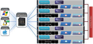
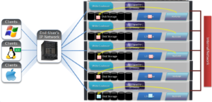
OneFS run equally across all the nodes in a cluster such that no one node controls the cluster and all nodes are true peers. Looking from a high-level at the components within each node, the I/O stack is split into a top layer, or initiator, and a bottom layer, or participant. This division is used as a logical model for the analysis of OneFS’ read and write paths.
At a physical-level, CPUs and memory cache in the nodes are simultaneously handling initiator and participant tasks for I/O taking place throughout the cluster. There are caches and a distributed lock manager that are excluded from the diagram below for simplicity’s sake.
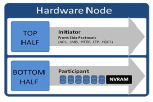
When a client connects to a node to write a file, it is connecting to the top half or initiator of that node. Files are broken into smaller logical chunks called stripes before being written to the bottom half or participant of a node (disk). Failure-safe buffering using a write coalescer is used to ensure that writes are efficient and read-modify-write operations are avoided. The size of each file chunk is referred to as the stripe unit size. OneFS stripes data across all nodes and protects the files, directories and associated metadata via software erasure-code or mirroring.
OneFS determines the appropriate data layout to optimize for storage efficiency and performance. When a client connects to a node, that node’s initiator acts as the ‘captain’ for the write data layout of that file. Data, erasure code (FEC) protection, metadata and inodes are all distributed on multiple nodes, and spread across multiple drives within nodes. The following illustration shows a file write occurring across all nodes in a three node cluster.
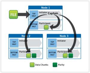
OneFS uses a cluster’s Ethernet or Infiniband back-end network to allocate and automatically stripe data across all nodes . As data is written, it’s also protected at the specified level.
When writes take place, OneFS divides data out into atomic units called protection groups. Redundancy is built into protection groups, such that if every protection group is safe, then the entire file is safe. For files protected by FEC, a protection group consists of a series of data blocks as well as a set of parity blocks for reconstruction of the data blocks in the event of drive or node failure. For mirrored files, a protection group consists of all of the mirrors of a set of blocks.
OneFS is capable of switching the type of protection group used in a file dynamically, as it is writing. This allows the cluster to continue without blocking in situations when temporary node failure prevents the desired level of parity protection from being applied. In this case, mirroring can be used temporarily to allow writes to continue. When nodes are restored to the cluster, these mirrored protection groups are automatically converted back to FEC protected.
During a write, data is broken into stripe units and these are spread across multiple nodes as a protection group. As data is being laid out across the cluster, erasure codes or mirrors, as required, are distributed within each protection group to ensure that files are protected at all times.
One of the key functions of the OneFS AutoBalance job is to reallocate and balance data and, where possible, make storage space more usable and efficient. In most cases, the stripe width of larger files can be increased to take advantage of new free space, as nodes are added, and to make the on-disk layout more efficient.
The initiator top half of the ‘captain’ node uses a modified two-phase commit (2PC) transaction to safely distribute writes across the cluster, as follows:
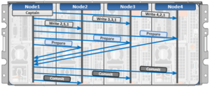
Every node that owns blocks in a particular write operation is involved in a two-phase commit mechanism, which relies on NVRAM for journaling all the transactions that are occurring across every node in the storage cluster. Using multiple nodes’ NVRAM in parallel allows for high-throughput writes, while maintaining data safety against all manner of failure conditions, including power failures. In the event that a node should fail mid-transaction, the transaction is restarted instantly without that node involved. When the node returns, it simply replays its journal from NVRAM.
In a write operation, the initiator also orchestrates the layout of data and metadata, the creation of erasure codes, and lock management and permissions control. OneFS can also optimize layout decisions made by to better suit the workflow. These access patterns, which can be configured at a per-file or directory level, include:
- Concurrency: Optimizes for current load on the cluster, featuring many simultaneous clients.
- Streaming: Optimizes for high-speed streaming of a single file, for example to enable very fast reading with a single client.
- Random: Optimizes for unpredictable access to the file, by adjusting striping and disabling the use of prefetch.
OneFS Multi-writer
In the previous blog article we took a look at write locking and shared access in OneFS. Next, we’ll delve another layer deeper into OneFS concurrent file access.
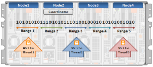
The OneFS locking hierarchy also provides a mechanism called Multi-writer, which allows a cluster to support concurrent writes from multiple client writer threads to the same file. This granular write locking is achieved by sub-diving the file into separate regions and granting exclusive data write locks to these individual ranges, as opposed to the entire file. This process allows multiple clients, or write threads, attached to a node to simultaneously write to different regions of the same file.
Concurrent writes to a single file need more than just supporting data locks for ranges. Each writer also needs to update a file’s metadata attributes such as timestamps, block count, etc. A mechanism for managing inode consistency is also needed, since OneFS is based on the concept of a single inode lock per file.
In addition to the standard shared read and exclusive write locks, OneFS also provides the following locking primitives, via journal deltas, to allow multiple threads to simultaneously read or write a file’s metadata attributes:
OneFS Lock Types include:
Exclusive: A thread can read or modify any field in the inode. When the transaction is committed, the entire inode block is written to disk, along with any extended attribute blocks.
Shared: A thread can read, but not modify, any inode field.
DeltaWrite: A thread can modify any inode fields which support delta-writes. These operations are sent to the journal as a set of deltas when the transaction is committed.
DeltaRead: A thread can read any field which cannot be modified by inode deltas.
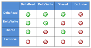
These locks allow separate threads to have a Shared lock on the same LIN, or for different threads to have a DeltaWrite lock on the same LIN. However, it is not possible for one thread to have a Shared lock and another to have a DeltaWrite. This is because the Shared thread cannot perform a coherent read of a field which is in the process of being modified by the DeltaWrite thread.
The DeltaRead lock is compatible with both the Shared and DeltaWrite lock. Typically the file system will attempt to take a DeltaRead lock for a read operation, and a DeltaWrite lock for a write, since this allows maximum concurrency, as all these locks are compatible.
Here’s what the write lock incompatibilities looks like:
OneFS protects data by writing file blocks (restriping) across multiple drives on different nodes. The Job Engine defines a ‘restripe set’ comprising jobs which involve file system management, protection and on-disk layout. The restripe set contains the following jobs:
- AutoBalance & AutoBalanceLin
- FlexProtect & FlexProtectLin
- MediaScan
- MultiScan
- SetProtectPlus
- SmartPools
- Upgrade
Multi-writer for restripe allows multiple restripe worker threads to operate on a single file concurrently. This in turn improves read/write performance during file re-protection operations, plus helps reduce the window of risk (MTTDL) during drive Smartfails, etc. This is particularly true for workflows consisting of large files, while one of the above restripe jobs is running. Typically, the larger the files on the cluster, the more benefit multi-writer for restripe will offer.
Note that OneFS multi-writer ranges are not a fixed size and instead tied to layout/protection groups. So typically in the megabytes size range. The number of threads that can write to the same file concurrently, from the filesystem perspective, is only limited by file size. However, NFS file handle affinity (FHA) comes into play from the protocol side, and so the default is typically eight threads per node.
The clients themselves do not apply for granular write range locks in OneFS, since multi-writer operation is completely invisible to the protocol. Multi-writer uses proprietary locking which OneFS performs to coordinate filesystem operations. As such, multi-writer is distinct from byte-range locking that application code would call, or even oplocks/leases which the client protocol stack would call.
Depending on the workload, multi-writer can improve performance by allowing for more concurrency, and (while typically on by default in recent releases) can be enabled on a cluster from the CLI as follows:
# isi_sysctl_cluster efs.bam.coalescer.multiwriter=1
Similarly, to disable multi-writer:
# isi_sysctl_cluster efs.bam.coalescer.multiwriter=0
Note that, as a general rule, unnecessary contention should be avoided. For example:
- Avoid placing unrelated data in the same directory: Use multiple directories instead. Even if it is related, split it up if there are many entries.
- Use multiple files: Even if the data is ultimately related, from a performance/scalability perspective, having each client use its own file and then combining them as a final stage is the correct way to architect for performance.
With multi-writer for restripe, an exclusive lock is no longer required on the LIN during the actual restripe of data. Instead, OneFS tries to use a delta write lock to update the cursors used to track which parts of the file need restriping. This means that a client application or program should be able to continue to write to the file while the restripe operation is underway.
An exclusive lock is only required for a very short period of time while a file is set up to be restriped. A file will have fixed widths for each restripe lock, and the number of range locks will depend on the quantity of threads and nodes which are actively restriping a single file.
OneFS File Locking and Concurrent Access
There has been a bevy of recent questions around how OneFS allows various clients attached to different nodes of a cluster to simultaneously read from and write to the same file. So it seemed like a good time for a quick refresher on some of the concepts and mechanics behind OneFS concurrency and distributed locking.
File locking is the mechanism that allows multiple users or processes to access data concurrently and safely. For reading data, this is a fairly straightforward process involving shared locks. With writes, however, things become more complex and require exclusive locking, since data must be kept consistent.
OneFS has a fully distributed lock manager that marshals locks on data across all the nodes in a storage cluster. This locking manager is highly extensible and allows for multiple lock types to support both file system locks as well as cluster-coherent protocol-level locks, such as SMB share mode locks or NFS advisory-mode locks. OneFS also has support for delegated locks such as SMB oplocks and NFSv4 delegations.
Every node in a cluster is able to act as coordinator for locking resources, and a coordinator is assigned to lockable resources based upon a hashing algorithm. This selection algorithm is designed so that the coordinator almost always ends up on a different node than the initiator of the request. When a lock is requested for a file, it can either be a shared lock or an exclusive lock. A shared lock is primarily used for reads and allows multiple users to share the lock simultaneously. An exclusive lock, on the other hand, allows only one user access to the resource at any given moment, and is typically used for writes. Exclusive lock types include:
Mark Lock: An exclusive lock resource used to synchronize the marking and sweeping processes for the Collect job engine job.
Snapshot Lock: As the name suggests, the exclusive snapshot lock which synchronizes the process of creating and deleting snapshots.
Write Lock: An exclusive lock that’s used to quiesce writes for particular operations, including snapshot creates, non-empty directory renames, and marks.
The OneFS locking infrastructure has its own terminology, and includes the following definitions:
Domain: Refers to the specific lock attributes (recursion, deadlock detection, memory use limits, etc) and context for a particular lock application. There is one definition of owner, resource, and lock types, and only locks within a particular domain may conflict.
Lock Type: Determines the contention among lockers. A shared or read lock does not contend with other types of shared or read locks, while an exclusive or write lock contends with all other types. Lock types include:
• Advisory
• Anti-virus
• Data
• Delete
• LIN
• Mark
• Oplocks
• Quota
• Read
• Share Mode
• SMB byte-range
• Snapshot
• Write
Locker: Identifies the entity which acquires a lock.
Owner: A locker which has successfully acquired a particular lock. A locker may own multiple locks of the same or different type as a result of recursive locking.
Resource: Identifies a particular lock. Lock acquisition only contends on the same resource. The resource ID is typically a LIN to associate locks with files.
Waiter: Has requested a lock, but has not yet been granted or acquired it.
Here’s an example of how threads from different nodes could request a lock from the coordinator:
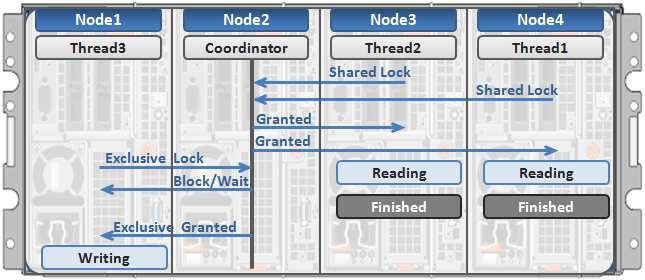
1. Node 2 is selected as the lock coordinator of these resources.
2. Thread 1 from Node 4 and thread 2 from Node 3 request a shared lock on a file from Node 2 at the same time.
3. Node 2 checks if an exclusive lock exists for the requested file.
4. If no exclusive locks exist, Node 2 grants thread 1 from Node 4 and thread 2 from Node 3 shared locks on the requested file.
5. Node 3 and Node 4 are now performing a read on the requested file.
6. Thread 3 from Node 1 requests an exclusive lock for the same file as being read by Node 3 and Node 4.
7. Node 2 checks with Node 3 and Node 4 if the shared locks can be reclaimed.
8. Node 3 and Node 4 are still reading so Node 2 asks thread 3 from Node 1 to wait for a brief instant.
9. Thread 3 from Node 1 blocks until the exclusive lock is granted by Node 2 and then completes the write operation.
OneFS Drive Performance Statistics
The previous post examined some of the general cluster performance metrics. In this article we’ll focus in on the disk subsystem and take a quick look at some of the drive statistics counters. As we’ll see, OneFS offers several tools to inspect and report on both drive health and performance.
Let’s start with some drive failure and wear reporting tools….
The following cluster-wide command will indicate any drives that are marked as smartfail, empty, stalled, or down:
# isi_for_array -sX 'isi devices list | egrep -vi “healthy|L3”'
Usually, any node that requires a drive replacement will have an amber warning light on the front display panel. Also, the drive that needs swapping out will typically be marked by a red LED.
Alternatively, isi_drivenum will also show the drive bay location of each drive, plus a variety of other disk related info, etc.
# isi_for_array -sX ‘isi_drivenum –A’
This next command provides drive wear information for each node’s flash (SSD) boot drives:
# isi_for_array -sSX "isi_radish -a /dev/da* | grep -e FW: -e 'Percent Life' | grep -v Used”
However, the output is in hex. This can be converted to a decimal percent value using the following shell command, where <value> is the raw hex output:
# echo "ibase=16; <value>" | bc
Alternatively, the following perl script will also translate the isi_radish command output from hex into comprehensible ‘life remaining’ percentages:
#!/usr/bin/perl

use strict;

use warnings;

my @drives = ('ada0', 'ada1');

foreach my $drive (@drives)

{

print "$drive:\n";

open CMD,'-|',"isi_for_array -s isi_radish -vt /dev/$drive" or

die "Failed to open pipe!\n";

while (<CMD>)

{

if (m/^(\S+).*(Life Remaining|Lifetime Left).*\(raw\s+([^)]+)/i)

{

print "$1 ".hex($3)."%\n";

}

}

}
The following drive statistics can be useful for both performance analysis and troubleshooting purposes.
General disk activity stats are available via the isi statistics command.
For example:
# isi statistics system –-nodes=all --oprates --nohumanize
This output will give you the per-node OPS over protocol, network and disk. On the disk side, the sum of DiskIn (writes) and DIskOut (reads) gives the total IOPS for all the drives per node.
For the next level of granularity, the following drive statistics command provides individual SSSD drive info. The sum of OpsIn and OpsOut is the total IOPS per drive in the cluster.
# isi statistics drive -nall -–long --type=sata --sort=busy | head -20
And the same info for SSDs:
# isi statistics drive -nall --long --type=ssd --sort=busy | head -20
The primary counters of interest in drive stats data are often the ‘TimeInQ’, ‘Queued’, OpsIn, OpsOut, and IO and the ’Busy’ percentage of each disk. If most or all the drives have high busy percentages, this indicates a uniform resource constraint, and there is a strong likelihood that the cluster is spindle bound. If, say, the top five drives are much busier than the rest, this suggests a workflow hot-spot.
# isi statistics pstat
The read and write mix, plus metadata operations, for a particular protocol can be gleaned from the output of the isi statistics pstat command. In addition to disk statistics, CPU and network stats are also provided. The –protocol parameter is used to specify the core NAS protocols such as NFSv3, NFSv4, SMB1, SMB2, HDFS, etc. Additionally, OneFS specific protocol stats, including job engine (jobd), platform API (papi), IRP, etc, are also available.
For example, the following will show NFSv3 stats in a ‘top’ format, refreshed every 6 seconds by default:
# isi statistics pstat --protocol nfs3 --format top
The uptime command provides system load average for 1, 5, and 15 minute intervals, and is comprised of both CPU queues and disk queues stats.
# isi_for_array -s 'uptime'
It’s worth noting that this command’s output does not take CPU quantity into account. As such, a load average of 1 on a single CPU means the node is pegged. However, that load average of 1 on a dual CPU system means the CPU is 50% idle.
The following command will give the CPU count:
# isi statistics query current --nodes all --degraded --stats node.cpu.count
The sum of disk ops across a cluster per node is available via the following syntax:
# isi statistics query current --nodes=all --stats=node.disk.xfers.rate.sum
There are a whole slew of more detailed drive metrics that OneFS makes available for query.
Disk time in queue provides an indication as to how long an operation is queued on a drive. This indicator is key if a cluster is disk-bound. A time in queue value of 10 to 50 milliseconds is concerning, whereas a value of 50 to 100 milliseconds indicates a potential problem.
The following CLI syntax can be used to obtain the maximum, minimum, and average values for disk time in queue for SATA drives in this case:
# isi statistics drive --nodes=all --degraded --no-header --no-footer | awk ' /SATA/ {sum+=$8; max=0; min=1000} {if ($8>max) max=$8; if ($8<min) min=$8} END {print “Min = “,min; print “Max = “,max; print “Average = “,sum/NR}’
The following command displays the time in queue for 30 drives sorted highest-to-lowest:
# isi statistics drive list -n all --sort=timeinq | head -n 30
Queue depth indicates how many operations are queued on drives. A queue depth of 5 to 10 is considered heavy queuing.
The following CLI command can be used to obtain the maximum, minimum, and average values for disk queue depth of SATA drives. If there’s a big delta between the maximum number and average number in the queue, it’s worth investigating further to determine whether an individual drive is working excessively.
# isi statistics drive --nodes=all --degraded --no-header --no-footer | awk ' /SATA/ {sum+=$9; max=0; min=1000} {if ($9>max) max=$9; if ($9<min) min=$9} END {print “Min = “,min; print “Max = “,max; print “Average = “,sum/NR}’
For information on SAS or SSD drives, you can substitute SAS or SSD for SATA in the above syntax.
To display queue depth for twenty drives sorted highest-to-lowest, run the following command:
# isi statistics drive list -n all --sort=queued | head -n 20
Note that the TimeAvg metric, as reported by isi statistics drive command, represents all the latency at the disk that doesn’t include the scheduler wait time (TimeInQ). So this is a measure of disk access time (ie. send the op, wait, receive response). The Total Time at the disk is a sum of the access time (TimeAvg) and the scheduler time (TimeInQ).
The disk percent busy metric can he useful to determine if a drive is getting pegged. However, it does not indicate how much extra work may be in the queue. To obtain the maximum, minimum, and average disk busy values for SATA drives, run the following command. For information on SAS or SSD drives, you can include SAS or SSD respectively, instead of SATA.
# isi statistics drive --nodes=all --degraded --no-header --no-footer | awk ' /SATA/ {sum+=$10; max=0; min=1000} {if ($10>max) max=$10; if ($10min) min=$10} END {print “Min = “,min; print “Max = “,max; print “Average = “,sum/NR}’
To display disk percent busy for twenty drives sorted highest-to-lowest issue, run the following command.
# isi statistics drive -nall --output=busy | head -n 20
OneFS Performance Statistics
There have been several recent inquiries on how to effectively gather performance statistics on a cluster, so it seemed like a useful topic to dig into further in a blog article:
First, two cardinal rules… Before planning or undertaking any performance tuning on a cluster, or its attached clients:
1) Record the original cluster settings before making any configuration changes to OneFS or its data services.
2) Measure and analyze how the various workloads in your environment interact with and consume storage resources.
Performance measurement is done by gathering statistics about the common file sizes and I/O operations, including CPU and memory load, network traffic utilization, and latency. To obtain key metrics and wall-clock timing data for delete, renew lease, create, remove, set userdata, get entry, and other file system operations, connect to a node via SSH and run the following command as root to enable the vopstat system control:
# sysctl efs.util.vopstats.record_timings=1
After enabling vopstats, they can be viewed by running the ‘sysctl efs.util.vopstats’ command as root: Here is an example of the command’s output:
# sysctl efs.util.vopstats.

efs.util.vopstats.ifs_snap_set_userdata.initiated: 26

efs.util.vopstats.ifs_snap_set_userdata.fast_path: 0

efs.util.vopstats.ifs_snap_set_userdata.read_bytes: 0

efs.util.vopstats.ifs_snap_set_userdata.read_ops: 0

efs.util.vopstats.ifs_snap_set_userdata.raw_read_bytes: 0

efs.util.vopstats.ifs_snap_set_userdata.raw_read_ops: 0

efs.util.vopstats.ifs_snap_set_userdata.raw_write_bytes: 6432768

efs.util.vopstats.ifs_snap_set_userdata.raw_write_ops: 2094

efs.util.vopstats.ifs_snap_set_userdata.timed: 0

efs.util.vopstats.ifs_snap_set_userdata.total_time: 0

efs.util.vopstats.ifs_snap_set_userdata.total_sqr_time: 0

efs.util.vopstats.ifs_snap_set_userdata.fast_path_timed: 0

efs.util.vopstats.ifs_snap_set_userdata.fast_path_total_time: 0

efs.util.vopstats.ifs_snap_set_userdata.fast_path_total_sqr_time: 0
The time data captures the number of operations that cross the OneFS clock tick, which is 10 milliseconds. Independent of the number of events, the total_sq_time provides no actionable information because of the granularity of events.
To analyze the operations, use the total_time value instead. The following example shows only the total time records in the vopstats:
# sysctl efs.util.vopstats | grep –e "total_ time: [ ^0]"

efs.util.vopstats.access_rights.total_time: 40000

efs.util.vopstats.lookup.total_time:  30001

efs.util.vopstats.unlocked_ write_mbuf.total_time:  340006

efs.util.vopstats.unlocked_write_mbuf.fast_path_total_time: 340006

efs.util.vopstats.commit.total_time: 3940137

efs.util.vopstats.unlocked_getattr.total_time: 280006

efs.util.vopstats.unlocked_getattr.fast_path_total_time:   50001 efs.util.vopstats.inactive.total_time: 100004

efs.util.vopstats.islocked.total_time:   30001 efs.util.vopstats.lock1.total_time:   280005

efs.util.vopstats.unlocked_read_mbuf.total_time: 11720146 efs.util.vopstats.readdir.total_time: 20000

efs.util.vopstats.setattr.total_time: 220010 efs.util.vopstats.unlock.total_time: 20001

efs.util.vopstats.ifs_snap_delete_resume.timed: 77350

efs.util.vopstats.ifs_snap_delete_resume.total_time: 720014

efs.util.vopstats.ifs_snap_delete_resume.total_sqr_time: 7200280042
The ‘isi statistics’ CLI command is a great tool for the task here, plus its output is current (ie. real time). It’s a versatile utility, providing real time stats with the following subcommand-level syntax
| Statistics
Category |
Details |
| Client | Display cluster usage statistics organized according to cluster hosts and users |
| Drive | Show performance by drive |
| Heat | Identify the most accessed files/directories |
| List | List valid arguments to given option |
| Protocol | Display cluster usage statistics organized by communication protocol |
| Pstat | Generate detailed protocol statistics along with CPU, OneFS, network & disk stats |
| Query | Query for specific statistics. There are current and history modes |
| System | Display general cluster statistics (Op rates for protocols, network & disk traffic (kB/s) |
Full command syntax and a description of the options can be accessed via isi statistics –help or via the man page (man isi-statistics).
The ‘isi statistics pstat’ command provides statistics per protocol operation, client connections, and the file system. For example, for NFSv3:
# isi statistics pstat --protocol=nfs3
The ‘isi statistics client’ CLI command provides I/O and timing data by client name and/or IP address, depending on options – plus the username if it can be determined. For example, to generate a list of the top NFSv3 clients on a cluster, the following command can be used:
# isi statistics client --protocols=nfs3 –-format=top
Or, for SMB clients:
# isi statistics client --protocols=smb2 –-format=top
The extensive list of protocols for which client data can be displayed includes:
nfs3 | smb1 | nlm | ftp | http | siq | smb2 | nfs4 | papi | jobd | irp | lsass_in | lsass_out | hdfs | all | internal | external
SMB2 and SMB3 current connections are both displayed in the following stats command:
# isi statistics query current --stats node.clientstats.active.smb2
Or for SMB2 + 3 historical connection data:
# isi statistics query history --stats node.clientstats.active.smb2
The following command will total by users, as opposed to node. This can be helpful when investigating HPC workloads, or other workflows involving compute clusters:
# isi statistics client --protocols=nfs3 –-format=top --numeric --totalby=username --sort=ops,timemax
This ‘heat’ command option can be useful for viewing the files that are being utilized:
# isi statistics heat --long --classes=read,write,namespace_read,namespace_write | head -10
This shows the amount of contention where parallel user(s) operations are targeting the same object.
# isi statistics heat --long --classes=read,write,namespace_read,namespace_write --events=blocked,contended,deadlocked | head -10
It can also be useful to constrain statistics reporting to a single node. For example, the following command will show the fifteen hottest files on node 4.
# isi statistics heat --limit=15 --nodes=4
It’s worth noting that isi statistics doesn’t directly tie a client to a file or directory path. Both isi statistics heat and isi statistics client provide some of this information, but not together. The only directory/file related statistics come from the ‘heat’ stats, which track the hottest accesses in the filesystem.
The system and drive statistics can also be useful for performance analysis and troubleshooting purposes. For example:
# isi statistics system -–nodes=all --oprates --nohumanize
This output will give you the per-node OPS over protocol, network and disk. On the disk side, the sum of DiskIn (writes) and DIskOut (reads) gives the total IOPS for all the drives per node.
For the next level of granularity, the drive statistics command provides individual disk info.
# isi statistics drive -nall -–long --type=sata --sort=busy | head -20
If most or all the drives have high busy percentages, this indicates a uniform resource constraint, and there is a strong likelihood that the cluster is spindle bound. If, say, the top five drives are much busier than the rest, this would suggest a workflow hot-spot.
OneFS Time Synchronization & NTP
OneFS provides a network time protocol (NTP) service to ensure that all nodes in a cluster can easily be synchronized to the same time source. This service automatically adjusts a cluster’s date and time settings to that of one or more external NTP servers.
NTP configuration on a cluster is performed by using the ‘isi ntp’ command line (CLI) utility, rather than modifying the nodes’ /etc/ntp.conf files manually. The syntax for this command is divided into two parts: servers and settings. For example:
# isi ntp settings

Description:

    View and modify cluster NTP configuration.

Required Privileges:

    ISI_PRIV_NTP

Usage:

    isi ntp settings <action>

        [--timeout <integer>]

        [{--help | -h}]

Actions:

    modify    Modify cluster NTP configuration.

    view      View cluster NTP configuration.

Options:

  Display Options:

    --timeout <integer>

        Number of seconds for a command timeout (specified as 'isi --timeout NNN

        <command>').

    --help | -h

        Display help for this command.
There is also an isi_ntp_config CLI command available in OneFS that provides a richer configuration set and combines the server and settings functionality :
Usage: isi_ntp_config COMMAND [ARGUMENTS ...]

Commands:

    help

      Print this help and exit.

    list

      List all configured info.

    add server SERVER [OPTION]

      Add SERVER to ntp.conf.  If ntp.conf is already

      configured for SERVER, the configuration will be replaced.

      You can specify any server option. See NTP.CONF(5)


    delete server SERVER

      Remove server configuration for SERVER if it exists.


    add exclude NODE [NODE...]

      Add NODE (or space separated nodes) to NTP excluded entry.

      Excluded nodes are not used for NTP communication with external

      NTP servers.


    delete exclude NODE [NODE...]

      Delete NODE (or space separated Nodes) from NTP excluded entry.


    keyfile KEYFILE_PATH

      Specify keyfile path for NTP auth. Specify "" to clear value.

      KEYFILE_PATH has to be a path under /ifs.


    chimers [COUNT | "default"]

      Display or modify the number of chimers NTP uses.

      Specify "default" to clear the value.
By default, if the cluster has more than three nodes, three of the nodes are selected as ‘chimers’. Chimers are nodes which can contact the external NTP servers. If the cluster comprises three nodes or less, only one node will be selected as a chimer. If no external NTP server is set, they will use the local clock instead. The other non-chimer nodes will use the chimer nodes as their NTP servers. The chimer nodes are selected by the lowest node number which is not excluded from chimer duty.
If a node is configured as a chimer. its /etc/ntp.conf entry will resemble:
# This node is one of the 3 chimer nodes that can contact external NTP

# servers. The non-chimer nodes will use this node as well as the other

# chimers as their NTP servers.

server time.isilon.com

# The other chimer nodes on this cluster:

server 192.168.10.150 iburst

server 192.168.10.151 iburst

# If none or bad connection to external servers this node may become

# the time server for this cluster. The system clock will be a time

# source and run at a high stratum
In addition to managing NTP servers and authentication, individual nodes can also be excluded from communicating with external NTP servers.
The local clock of the node is set as an NTP server at a high stratum level. In NTP, a server with lower stratum number is preferred, so if an external NTP server is set the system will prefer an external time server if configured. The stratum level for the chimer is determined by the chimer number. The first chimer is set to stratum 9, the second to stratum 11, and the others continue to increment the stratum number by 2. This is so the non-chimer nodes will prefer to get the time from the first chimer if available.
For a non-chimer node, its /etc/ntp.conf entry will resemble:
# This node is _not_ one of the 3 chimer nodes that can contact external

# NTP servers. These are the cluster's chimer nodes:

server 192.168.10.149 iburst true

server 192.168.10.150 iburst true

server 192.168.10.151 iburst true
When configuring NTP on a cluster, more than one NTP server can be specified to synchronize the system time from. This allows for full redundancy of ysnc targets. The cluster periodically contacts these server(s) and adjusts the time and/or date as necessary, based on the information it receives.
The ‘isi_ntp_config’ CLI command can be used to configure which NTP servers a cluster will reference. For example, the following syntax will add the server ‘time.isilon.com’:
# isi_ntp_config add server time.isilon.com
Alternatively, the NTP configuration can also be managed from the WebUI by browsing to Cluster Management > General Settings > NTP.
NTP also provides basic authentication-based security via symmetrical keys, if desired.
If no NTP servers are available, Windows Active Directory (AD) can synchronize domain members to a primary clock running on the domain controller(s). If there are no external NTP servers configured and the cluster is joined to AD, OneFS will use the Windows domain controller as the NTP time server. If the cluster and domain time become out of sync by more than 4 minutes, OneFS generates an event notification.
Be aware though, that if the cluster and Active Directory drift out of time sync by more than 5 minutes, AD authentication will cease to function.
If neither an NTP server or domain controller are available, the cluster’s time, date, and time zone can also be set manually using the ‘isi config’ CLI command. For example:
1. Run the ‘isi config’ command. The command-line prompt changes to indicate that you are in the isi config subsystem:
# isi config

Welcome to the Isilon IQ configuration console.

Copyright (c) 2001-2017 EMC Corporation. All Rights Reserved.

Enter 'help' to see list of available commands.

Enter 'help <command>' to see help for a specific command.

Enter 'quit' at any prompt to discard changes and exit.

        Node build: Isilon OneFS v8.2.2 B_8_2_2(RELEASE)Node serial number: JWXER170300301

>>>
2. Specify the current date and time by running the date command. For example, the following command sets the cluster time to 9:20 AM on April 23, 2020:
>>> date 2020/04/23 09:20:00

Date is set to 2020/04/23 09:20:00
3. The ‘help timezone’ command will list the available timezones. For example:
>>> help timezone


timezone [<timezone identifier>]


Sets the time zone on the cluster to the specified time zone.

Valid time zone identifiers are:

        Greenwich Mean Time

        Eastern Time Zone

        Central Time Zone

        Mountain Time Zone

        Pacific Time Zone

        Arizona

        Alaska

        Hawaii

        Japan

        Advanced
4. To verify the currently configured time zone, run the ‘timezone’ command. For example:
>>> timezone

The current time zone is: Greenwich Mean Time
5. To change the time zone, enter the timezone command followed by one of the displayed options. For example, the following command changes the time zone to Alaska:
>>> timezone Alaska

Time zone is set to Alaska
A message confirming the new time zone setting displays. If your desired time zone did not display when you ran the help timezone command, enter ‘timezone Advanced’. After a warning screen, you will proceed to a list of regions. When you select a region, a list of specific time zones for that region appears. Select the desired time zone (you may need to scroll), then enter OK or Cancel until you return to the isi config prompt.
6. When done, run the commit command to save your changes and exit isi config.
>>> commit

Commit succeeded.
Alternatively, these time and date parameters can also be managed from the WebUI by browsing to Cluster Management > General Settings > Date and Time.
Setting Up Share Host ACLs Isilon OneFS

How do you allow or deny host for SMB shares?
In Isilon’s OneFS administrators can set Host ACLs on SMB shares. Setting up theses ACLs can add an extra layer of security for files in a specific share. For example administrators can deny all traffic except from certain servers.
OneFS Setting Up Share Host ACLs Commands
Below are the commands used in the Setting Up Share Host ACLs demo. NASA refers to the SMB Share used deny all traffic except from the specific host or hosts.
List out all the shares specific zone
isi smb shares list
View specifics on particular share in access zone
isi smb shares view nasa
Modify Host ACLs on particular share in access zone
isi smb share modify nasa --add-acl
Clear Host ACLs on specific share
isi smb share modify nasa --clear-host-acl
or
isi smb share modify nasa --revert-host-acl
Video – Setting Up Host ACLs on Isilon File Share
Transcript
Hi, folks. Thomas Henson here with thomashenson.com. And today is another episode of Isilon Quick Tips. So, what we want to cover on today’s episode is I want to go in through the CLI, and look at some of the commands that we can do on isi shares. And specifically, I want to look at some of the advanced features. So, something around the ACLs where we can deny certain hosts or allow certain hosts, too. So, follow along with me right after this. [Music]. So, in today’s episode we want to look at SMB Shares, but specifically from the Command Line. What we’re really going to focus on as I open this Share here is some of these advanced settings. So, you can see that we have some of these advanced settings, like continuous availability of time. And it looks like that we can change some of these. But when we change them, we’re just going to type in how we want to change those here. So, if you wanted to, for example in the host ACL, be able to deny or allow certain hosts, this is where we can do that. But let’s find out how we can this from the Command Line. Because there is a couple of different options, and a couple ways we can do it, and specifically we want to learn how to do it from the Command Line. So, here we are. I’m log back in to my Command Line. So, you can see I’m on Isilon-2. So, the first command I want to do is I want to list out all those SMB Shares that we had. So, we had three of those. So, the command is that we’re going to use in is the smb shares. And I’m just going to type return, so we can see what those actions are. So, you can see that we can do a list, which is the first thing we want to do. But you can also create those shares, you can delete shares, and we can view specific properties on each one of those shares. So, going back in. Let’s run a list on our shares. And you can see… All right. So, we have all those shares that we were just looking at from our [INAUDIBLE 00:02:00]. One thing to note here is if you are using this shares list command and you don’t see your zones, make sure that you type in the zone here. So, we will type in a specific zone. So, if you didn’t see the shares, make sure that you’re specifying exactly what zone there is. I only have one zone in my lab environment here on the system, so I can see that all may shares are there. So, now that I know my shares are there, let’s go back. I want to look at the nasa share that we have. So, let’s use the view command NASA. And you can see here that it’s going to give me my permissions, but then also those advanced features that we were talking about, we can see those here. So, for example we have the Access Based Enumeration. So, if you’re looking to be able to hide files or folders for users that don’t have those permissions, you can see that if that set here. Then also the File Mask. So, you can see that on default directly in File Mask is 700. So, if you’re looking about [INAUDIBLE 00:02:54] the File Mask is, if you’re not familiar, that’s the default permissions that are set whenever you have a File Directory that’s created in this share. So, you can see that in mine, the default setting is 700. Then specifically, the one that I really want to go over was the Host ACL. So, you can see the Hos ACL. I don’t have anything set here. And this is the property we can change, that will allow or deny certain hosts to the specific share. So, one of the reasons this came up is we were trying to secure an application from a share, and we wanted to able to say, ͞Hey, it’s only going to accept traffic from two or one specific server, and then we’re going to deny all those.͟ So, what we’re going to do is I want to walk through how to do that. So specifically, we’re still going to use our isismb share. But now we’re going to use the modify. So, you see the isi smb share modify command. You can see that when we do that… I’m just going to show you some of the commands that we have here. But you can see we have a lot of different options we can do. But the first thing is, remember, we’re going to type in that share.
So, here I want to pass in my nasa string. I don’t have to pass in zone, because I only have one zone. But if you have different zones, then you’re going to want to pass that zone in. The command that we’re specifically looking for is this host-acl. So, we have some options here with the host-acl. We can clear the host, we can add a host, and we can remove a host. So, what we want to do is we want to add a host that’s going to allow for host coming from. We’re just going to say 192.170.170.001. Then we’re going to deny our host from that. So, we’re going to clear this out, so we can have that at the top of the screen. So, you can see we have it here. So, that isi smb shares modify. Then you’re going to put in here you share name. So, mine is nasa. And we’re going to do –add-host-acl=, the first thing that we’re going to do is we’re going to allow. So, we’re going to allow traffic from 192.170.170.001 Then we’re going to use a comma to separate that out, and then we’re going to say that we’re going to deny all. So, specifically we could do this different, and say that we want to allow traffic from all and then deny from specific ones. But from this use case, and this is probably the most common one especially when you’re trying to lock down a certain share, you’re going to want to use this command. So, we’re typing the command, get the command prompt back again. And now let’s do that view. So, it’s view our nasa, and see if our changes are in there. So, you can see in our Host ACL, we have it. Then if we wanted to go back to our share from the [INAUDIBLE 00:05:43] and just see if those changes took. You can see in our advanced setting here, now it showing us are allow and deny all. Now, [INAUDIBLE 00:05:52] to say that I want to keep this going on my [INAUDIBLE 00:05:55] or if I want to revert back. So, there is a couple of different options. If you remember we had the clear-host-acl or the revert back. So, now I can just use this isi smb shares modify on my nasa directory. Once again, just as a reminder, use your own name if you have a specific zone. Then now I can revert my Host ACL. Now, we have that, I’m going to clear this out, and check. You can see our Host ACL is reverted back. We don’t have one set there. So, now we’re allowing traffic as long as you have the permissions to get to this file, and we don’t have one set. Well, that’s all for Isilon Quick Tips for today. Make sure to subscribe so that you never miss an episode of Isilon Quick Tips, or some of the other amazing contents that I have on my YouTube Channel here. And I will see you next time. [Music]
Isilon Quick Tips: Setting Up NFS Export in OneFS
Another Isilon Quick Tip, where I walk through setting up NFS export in OneFS. Setting up NFS exports is one of the baseline skills needed when working with OneFS.
NFS or Network File System is a protocol that allows file based access in a distributed environments. If you are familiar with Windows based systems it’s similar to the SMB protocol but mostly used in Linux/Unix environments. Chances are if you have any Linux/UNIX machines in your environment, you will have a need for using NFS exports.
When Do I Need an NFS Export?
Let’s jump into a couple use cases when you would want to mount an NFS export.
- Suppose you need extra capacity on your local machine
- Offload archive data to a network based file system
- Allow for file sharing abilities for a group of users
- Manage file access across a in a distributed environment
- Large data transfers or access to large files across network
Setting Up NFS Export in OneFS
- Open OneFS WebGUI
- Navigate to Protocols –> UNIX Sharing (NFS)
- Click Create Export
- Select directory to be shared
- Click Create Export
- Mount NFS export on Linux/UNIX machine (see commands below)
Transcript
In this episode of Isilon Quick Tips, we’re going to focus on accessing NFS Exports from Isilon’s OneFS.
If you’re accessing Isilon from a Linux machine, you’ll want to make use of the network file system—or NFS—protocol. To do this, we’ll be using mount commands. But first, let’s set up a directory that we want to share out through an NFS export. All this will be done from OneFS web interface and a Linux command line. So, follow along.
From our Protocol tab, we’ll go to the UNIX Sharing or NFS. Within our NFS Exports, we’ll have one defaulted, and that default will be for our IFS directory. Remember, anything in that IFS directory is everything that’s in Isilon. So, that’s one that’s set up by default, but let’s set up one that is specific just to maybe our data. So, I’m going to create an export. We can select our path and we can go down as deep as we want. So, I could go into our data and do something off the home shares or some of the archive data. But I just want to set a top-level directory for just our data path and share this one out. So, I’m going to select ifs/data, and then this is all of our data in Isilon. You don’t have to set a description. It’s just good once you start managing quite a few of these. You want to be like, okay, you can look at it and say, “Hey, okay, that’s actually what this export supports.” With our permissions, we can restrict it to read-only, but we don’t want to do that because we want to be able to make this a working directory. But I will click the “Enable mount access to subdirectories.” So, we’re not only accessing that data – we’re actually accessing everything inside of data and all the subdirectories involved as well. From here, I’ll just create my export, and we get a green check, which means we’re good to go. We now have two exports available. We have one from our IFS and one from our data. So, now we’ll need to jump back into a Linux box and access this from the command line.
So, from our Linux machine, I’m just going to show my directory path. So, I’m here in the root directory and I’ve got some files here. The first thing I want to do—and one of the ways that I always troubleshoot setting up the NFS mounts—is let’s see what mounts are available. So, we’re going to run a showmount command, and what we’re expecting to see is that IFS export, and also the IFS data that we just set up. So, the syntax is just showmount -e, and it’s going to be our Isilon cluster name. So, I’ve just got an IP address for mine. All right, and just like we expected, we see our IFS data, and then our IFS, and those are both accessible to us. Now all we have to do is create a directory to put this in. So, from our root directory, I’m just going to use an mkdir, and let’s set up a directory called our data-share. Just confirm that it’s there. And now we’ll just that mount command. So, mount [Isilon cluster name]:, which export we’re going to use. Remember, we’re going to use the IFS data, but you could use the IFS and mount to all the data that’s in Isilon. Now we need to put the full path of the directory that we want to put it in. So, we just created the data-share, and then now we should be able to run LS on our data-share. And now we see that we have our data in here. So, we have our Isilon support, we have project data, we have that home share data and that archive data – all mounted here.
So, this is a quick way just to set up an NFS export from a Linux machine to your Isilon cluster. Thanks for joining me for another Isilon Quick Tip.