PowerScale & Isilon – Page 7 – Unstructured Data Quick Tips

OneFS and Externally Managed Network Pools – Management and Monitoring

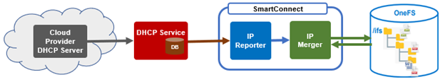
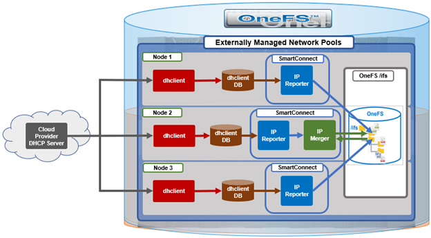
In the first article in this series, we took a look at the overview and architecture of the OneFS 9.7 externally managed network pools feature. Now, we’ll turn our focus to its management and monitoring.

From a cluster security point of view, the externally managed IP service has opened up a potential new attack vector whereby a rogue DHCP server could provide bad data. As such, the recommendation is to configure a firewall around this new OneFS DHCP service to ensure that the cluster is protected. While the OneFS firewall could in theory provide this protection, in order to know what the DHCP server is, the cluster first has to discover and talk to the DHCP server and get its IP. This seems a bit paradoxical (and insecure) to be creating a firewall rule after having already talked to and trusted the DHCP server.

The following table contains recommended configuration settings for the AWS firewall.

Setting	Value
Name	Eg. ‘DHCP”
Type	‘ingress’
From Port	67
To Port	68
Protocol	UDP
CIDR Blocks	<cluster_gateway>/32
IPv6 CIDR Blocks	[]
Security Group ID	// customer specific

Note that, as mentioned in the first article in this series, there are a currently a couple of instances of unsupported networking functionality in the APEX file services for AWS offering, as compared to on-prem OneFS, and these include:

IPv6 support
VLANs
Link aggregation
NFSoverRDMA

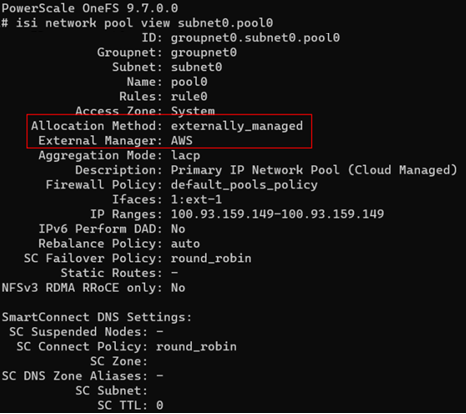
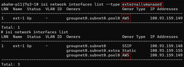
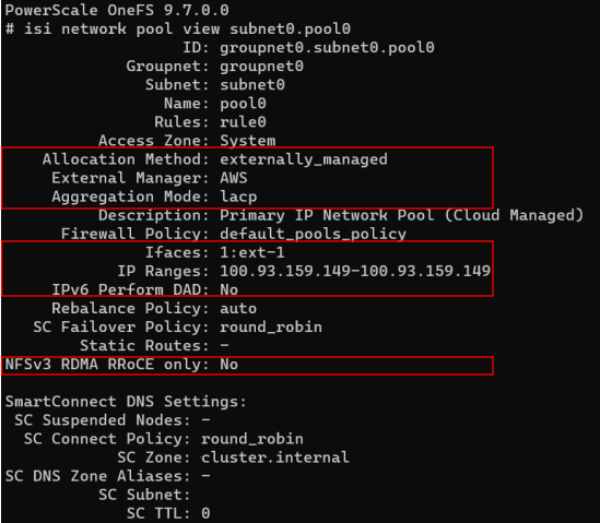
These limitations for externally managed network pools are highlighted in red below, and are read-only settings since they are managed by the cloud provider (interfaces and IPs).

Externally managed network pools can only be created by the system with OneFS 9.7 and therefore pools cannot be manually reconfigured either to or from externally managed – even by root.

In general manual IP configuration is protected in order to guard against accidental misconfiguration. However, clusters admin may occasionally be required to manually configure the IPs in the network pool, and can be performed with the ‘isi network pool modify’ plus the inclusion of the ‘–force’ flag:

# isi network pool modify subnet0.pool0 –ranges <ip_add_range> --force

Note that AWS has a maximum threshold for the number of IPs that can be configured per network interface based on AMI instance type. If this limit is exceeded, AWS will prevent the IP address from being configured, resulting in a potential data unavailability event. OneFS 9.7 now prevents most instances of IP oversubscription at configuration time in order to ensure availability during a 1/3 cluster outage.

While OneFS accounts for externally managed, static, dynamic IPs, and SSIPs, it is unable to account for unevenly allocated dynamic IPs, so it’s therefore unable to prevent all instances.

OneFS also displays an informative error message if attempting to configure this. For example, using an AMI instance type of ‘m5d.large’:

# isi network pool modify subnet0.pool0 –ranges 10.20.30.203-10.20.30.254

AWS only allows node 2 (instance type AWS=m5d.large) to have a maximum of 10 IPv4 addresses configured. In a degraded state, the requested configuration will result in node 2 attempting to configure 28 addresses, which will leave 18 address(es) unavailable. To resolve this, consider increasing the number of nodes in dynamic pools or reducing the number of IPv4 addresses.

When it comes to troubleshooting externally managed pools, there are two log files which are useful to check. Namely:

/var/log/dhclient.log
/var/log/isi_smartconnect

The first of these is a dedicated dhclient.log file for the new dhclient instance that OneFS 9.7 introduces. In contrast, the IP Merger and IP Reporter modules will output to the isi_smartconnect log.

There are also a handful of relevant system files that are also worth being aware of, and these include:

/var/db/dhclient/lease.ena1
/ifs/.ifsvar/modules/flexnet/ip_reporter/DHCP/node.
/ifs/.ifsvar/modules/flexnet/pool_members/groupnet.1.subnet.1.pool.1
/ifs/.ifsvar/modules/smartconnect/resource/workers/ip_merger

The first of these, lease.ena1, is an append log maintained by dhclient. So the most recent lease in there is the one that is SmartConnect is looking at. Note that there may be other lease files in the system, but only the lease files in /var/db/dhclient are relevant, and being viewed by SmartConnect. OneFS has a special configuration for dhclient to ensure this.

The IP reports live in the /ifs/.ifsvar/modules/flexnet directory. The pool_members directory has been present in OneFS for a number of years now. And OneFS now coordinates the IP merger with the file under ./smartconnect/resource/workers/ directory.

As for useful CLI commands, these include the following:

# isi_smartconnect_client action –a wake-ip-reporter

The ‘isi_smartconnect_client’ CLI utility, which can be used to interact with the SmartConnect daemon, gets an additional ‘wake-ip-reporter’ action in OneFS 9.7. Under normal circumstances, the IP Reporter only checks the contents of the lease file every five minutes. However, ‘wake-ip-reporter’ now instructs IP Reporter to check the lease file immediately. So if there was some issue where dhclient restarted for some reason, IP Reporter can be awoken and forced to read the lease, rather than waiting for its next scheduled check.

Additionally, the following ‘log_level’ command arguments can be used to change the logging level of SmartConnect to the desired verbosity:

# isi_smartconnect_client log_level [-l | -r]

Note that, in OneFS 9.7, this does not change the Flexnet config file which was required in prior releases.

Instead, this log level is reset when the process dies or the ‘–r’ argument is passed. It’s worth noting that this command does not operate cluster-wise. Rather, it just affects the current instance of SmartConnect running on the local node.

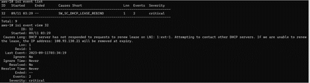
Another thing to be aware of when a cluster is using externally managed pools is that networking is dependent on, and can be impacted by, the availability of AWS’ DHCP servers. While the leased IP never changes, the leases themselves have an expiration of an hour. As such, if OneFS is unable to reach the DHCP server to renew, it may lose its Primary IPs. While this is often outside the realm of control, the OneFS CELOG event service will fire a critical warning alert (SW_SC_DHCP_LEASE_REBIND) before a primary IP expires. This alert will contain the following event description:

DHCP server has not responded to requests to renew lease on <interface>. Attempting to contact other DHCP servers. If we are unable to renew the lease, the IP address <ip_address> will be removed at expiry.

For example:

In addition to the above alert, there are several log messages that give a good indication of what may be amiss. These, and their resolution info, are summarized in the following table:

Log Message	Description	Resolution
Unable to merge IP 1.2.3.4 on ext-1 from devid 1 – no matching pool found	IP is not configured in any Network Pool	Add IP to the Primary IP Pool
Unable to parse lease on NIC: ena1. Attempting to retrieve new lease	The lease file generated by dhclient could not be read.	None should be required. We will automatically backup the old lease file and restart dhclient
Lease on NIC: ena1 not found	Lease file does not exist for the specified interface	OneFS will automatically restart dhclient
Unexpected error comparing IP Reports. Attempting rewrite	We try to dedupe writes by comparing newly generated IP report with what is on disk. In the event of a failure, we’ll just overwrite.
No IP Report received from DHCP External Manager	OneFS unable to determine its IP from the DHCP leases. Will continue retrying, but currently unable to report an IP	If issues persists, check on dhclient to ensure it is operating correctly.
Failed to write IP Report node. for DHCP to disk:	OneFS unable to report its IP to /ifs, so the IP merger is unable to update Flexnet/IP Assignments with this information.	Check why SmartConnect is unable to write to /ifs. Is it read only?

OneFS and Externally Managed Network Pools

Tucked amongst the array of new functionality within OneFS 9.7’s payload is the debut of a networking feature called externally managed network pools. In layman’s terms, this is essentially the introduction of a front-end dynamic host control protocol (DHCP) client for the PowerScale cluster.

The context and motivation behind implementing this new functionality is predicated on the fact that cloud networking differs substantially from on-prem infrastructure. This is largely because the cloud hyperscalers typically require a primary IP to be configured on a specific interface that they dictate. Normally, systems operating within an off-prem environment obtain their network configuration via the DHCP protocol. But as you’re likely aware, until OneFS 9.7, DHCP has not been supported on a cluster’s front end network previously. To support APEX file services for AWS, OneFS 9.6 implemented a manual work-around for this, which had its limitations. However, with OneFS 9.7, the desire was to make the system smarter and by adding proper support for IPv4 primary IP addresses on AWS deployments, thereby negating the need for configuring manual work-arounds, with their inherent risks.

This new externally managed IP addresses feature is automatically enabled upon committing and upgrade to OneFS 9.7. To support this feature, a new network allocation method has been added to OneFS’ network pools called ‘externally managed’. This is actually managed by an external service such as AWS, which dictates where these primary IPs live. So they are in charge of IP allocation, rather than the cluster’s Flexnet or SmartConnect services, which has been the case up to now. It’s worth noting that OneFS 9.7 only includes (and enforces) limited DHCP support, strictly for cloud deployments currently. That said, on-prem DHCP support may be added in a future release but this is currently not on the near-term roadmap. Additional work was also included in OneFS 9.7 to prevent IP oversubscription.

So let’s take a look under the hood… Architecturally, there are three main components to the externally managed IP addresses feature:

DHCP Service
IP Reporter Module
IP Merger Module

OneFS 9.7 actually talks DHCP by leveraging the FreeBSD ‘dhclient’ implementation. Dhclient is modified so it does not actually configure the network interfaces like it would normally, in order to avoid conflicts with the OneFS Flexnet network config daemon. Instead, dhclient just persists the leases to the following files:

/ifs/.ifsvar/modules/flexnet/flx_config.xml

/ifs/.ifsvar/modules/flexnet/pool_members/groupnet.1.subnet.1.pool.1.

Additionally, SmartConnect sees the addition of two new modules, IP Reporter and IP Merger.

Component	Details
DHCP service	Adds new MCP-controlled DHCP service: dhclient-ext-1 – Uses modified FreeBSD dhclient implementation – Does not configure network interfaces – Persists leases to /var/db/dhclient/
IP Merger	Adds new cluster-wide module to SmartConnect, IP Merger: – Coordinates ownership of the role by taking locks on files on /ifs – Loads all files from IP Reports directory – Verifies network pool is configured correctly and generates IP Assignments – Updates the following files: ▪ /ifs/.ifsvar/modules/flexnet/flx_config.xml ▪ /ifs/.ifsvar/modules/flexnet/pool_members/groupnet.1.subnet.1.pool.1
IP Reporter	Adds new module to each node’s SmartConnect service: – Parses DHCP leases – Converts to a generic format – Saves to /ifs/.ifsvar/modules/flexnet/ip_reports/DHCP/node.

These modules are still part of the overarching isi_smartconnect_d, and just new components within that same daemon. The IP Reporter module will parse the above lease files and then save the information to /ifs/.ifsvar/modules/flexnet/ip_reports/DHCP/node.

In contrast, the IP Merger is a single cluster-wide instance that loads the files from the IP Reports directory, verifies the network pool configuration, generates the IP assignments, and updates the config files. The ip_merger file contains the devID of the node that has been elected as responsible for IP merging. The full path is as follows:

/ifs/.ifsvar/modules/smartconnect/resource/workers/ip_merger

The following CLI syntax can be used to determine which node is acting as the merger: For example:

# isi_for_array 'grep "Taking ownership of the IPMerger role" /var/log/isi_smartconnect’

TME-4:  2024-02-07T16:26:20.946863+00:00 <3.6> GLaDOS-4(id4) isi_smartconnect_d[3626]: Taking ownership of the IPMerger role

In this case, the command output indicates that node ID4 has taken ownership of the IPMerger role.

The underlying process is very similar to how OneFS manages SSIPs in that all nodes attempt to lock a file under /ifs, and one granted that lock, they own that responsibility. So OneFS takes the files from under /ifs/.ifsvar/modules/flexnet/ip_reports and merges the IP information into the Flexnet config and the pool members file, as follows:

The above graphic illustrates how data flows through the system from the cloud provider’s DHCP server, to dhclient, and then into isi_smartconnect_d. The modular, extensible architecture requires only a small portion of OneFS to be made aware of this new type of network pool. This all happens on the side until the data is merged into the Flexnet config and the associated state files, so it is low risk to everything else.

In OneFS 9.7, this new DHCP allocation method is now set as ‘externally managed’ for subnet0.pool0. This can be seen even on network pools that have been upgraded from an earlier OneFS release. Additionally, the CLI output also reports the type of external manager for this network pool – for instance AWS in the example below:

The ‘isi network interfaces’ CLI syntax is also updated in OneFS 9.7 to allow filtering by ‘externally managed’ pools. For example below, again showing that the owner is AWS:

As a quick reminder, there are a currently a couple of instances of unsupported networking functionality in the APEX file services for AWS offering, as compared to on-prem OneFS, and these include:

IPv6 support
VLANs
Link aggregation
NFSoverRDMA

In the next article in this series we’ll turn our attention to the management, monitoring, and security of OneFS 9.7 externally managed network pools.

OneFS SmartSync Configuration for Google Cloud

As we saw in the previous blog in this series, with the inclusion of Google Cloud (GCP) in OneFS 9.7, SmartSync Cloud Copy now supports all three of the principal public cloud hyperscalers.

Object data replication to Google Cloud (GCP) can be configured in OneFS 9.7 via the ‘isi dm accounts create’ CLI command. Required information includes the regular account configuration parameters plus the following GCP-specific settings:

GCP account type
GCP URI
Access ID
Secret key

Or, more specifically:

Parameter	Description
Object store type	GCP (or AWS_S3, Azure, ECS_S3, etc)
URI	{http,https}://hostname:port/bucketname
Auth	Access ID, Secret Key
Proxy	Optional proxy information

For example:

# isi dm account create --account-type GCP --name [Account Name] --access-id [GCP access-id] --uri [GCP URI with bucket-name] --auth-mode CLOUD --secret-key [GCP secret-key]

Once created, the new account can be verified with the following command:

# isi dm accounts list

Additionally, the next steps for SmartSync configuration and policy creation are covered in detail in the following blog article.

SmartSync Cloud Copy supports both push and pull replication, permitting the same dataset that is copied to GCP with a push to be copied back to the cluster via a corresponding pull.

Be aware that a dataset must be available before a policy runs, or the policy will fail.

Also note that, while multiple GCP URIs and credentials are supported by SmartSync, they are not supported on the same account. Multiple accounts and multiple corresponding policies would need to be created for SmartSync.

Other SmartSync features and functionality includes:

Feature	Details
Bandwidth throttling	Set of netmask rules. Limits are per-node.
CPU throttling	Allowed and Back-off CPU percentages.
Base policies	Template providing common values to groups of related policies (schedule, source base path, enable/disable, etc). Ie. Disabling base policy affects all linked concrete policies.
Concrete policy	Predefined set of fields from the base policy
Unconnected nodes (NANON)	Active accounts are monitored by each node. No work allocation to nodes without network access.
Snapshot locking	Avoids accidental snapshot deletion, with subsequent re-base-lining.

Behind the scenes, dataset creation leverages a SnapshotIQ snapshot, which can be inspected via the ‘isi snapshot list’ command. These DM dataset snapshots are easily recognizable due to their ‘isi_dm’ prefixed naming convention.

The SmartSync Cloud Copy format provides both regular file representation, browsability and usability of file system data in the cloud. In addition to the replication of the actual data, SmartSync also preserves the common file attributes including Windows ACLs, POSIX permissions and attributes, creation times, extended attributes, etc. However, there are certain considerations and limitations to be aware of, such as no incremental copy. These also include:

CloudCopy Caveats	Details
ADS files	Skipped when encountered.
Hardlinks	An object will be created for each link (ie. links are not preserved).
Symlinks	Skipped when encountered.
Directories	An object is created for each directory.
Special files	Skipped when encountered.
Metadata	Only POSIX mode bits, UID, GID, atime, mtime, ctime are preserved.
Filename encodings	Converted to UTF-8.
Path	Path relative to root copy directory is used as object key.
Large files	An error is returned for files larger than the cloud providers maximum object size.
Long filenames	File names exceeding 256 bytes are compressed.
Long paths	Junction points are created when paths exceed 1024 bytes to redirect where objects are being stored
Sparse files	Sparse sections are not preserved and are written out fully as zeros.

SmartSync allows subsequent incremental data movement by managing and re-transferring failed file transfers. Similarly, Dataset reconnect enables systems with common base datasets to establish instant incremental syncs. SmartSync also proactively locks the SnapshotIQ snapshots it uses, providing better separation between Datamover and other snapshots.

Performance-wise, SmartSync is powered by a scalable run-time engine, spanning the cluster, and which spins up threads (fibers) on demand and uses asynchronous IO to process replication tasks (chunks). Batch operations are used for efficient small file, attribute, and data block transfer. Namespace contention avoidance, efficient snapshot utilization, and separation of dataset creation from transfer are salient design features of the both the baseline and incremental sync algorithms.

OneFS SmartSync and Google Cloud Support

Another feature addition that OneFS 9.7 delivers is support for Google Cloud (GCP) as a target for SmartSync, PowerScale’s next-gen data mover. With this enhancement, SmartSync Cloud Copy now supports all three of the principal public cloud hyperscalers – Amazon S3, Google Cloud Platform, and Microsoft Azure.

As you may be aware, this is not OneFS’ first foray into Google Cloud integration. CloudPools has supported GCP as a remote tiering target for several years now. Also, from the SmartSync perspective, while GCP represents a new account type, it fits within the existing cloud authentication mechanism, plus also uses an object protocol spec that’s based heavily on Amazon’s S3.

CloudCopy uses HTTP as the data replication transport layer to cloud storage, while traditional cluster to cluster SmartSync leverages a proprietary RCP-based messaging system.

In order to use SmartSync with GCP, the cluster must be running OneFS 9.7 and have SyncIQ licensed and active across all nodes in the cluster. Additionally, a cluster account with the ISI_PRIV_DATAMOVER privilege is needed in order to configure and run SmartSync data mover policies. While file-to-file replication requires SmartSync to be running on both source and target clusters, for OneFS Cloud Copy to transfer to/from cloud storage, only the cluster requires the SmartSync platform, and no data mover is required on the cloud systems. Be aware that the inbound TCP 7722 IP port must be open across any intermediate gateways and firewalls to allow SmartSync replication to occur.

Under the covers, replication is executed by the ‘isi_dm_d’ service, and the SmartSync data mover’s basic architecture is as follows:

The ‘isi_dm_d’ service is disabled by default and needs to be enabled prior to configuring and using SmartSync. SmartSync also uses TLS (transport layer security, or SSL) and, as such, requires trust to be established between the cluster and cloud target.

The SmartSync Datamover also includes a purpose-build, integrated scheduler and job control and execution framework, which operates along these lines:

Shared Key-Value Stores (KVS) are used for jobs/tasks distribution, and extra indexing is implemented for quick lookups by task state, task type, and alive time. There are no dependencies or communication between tasks, and job cancellation and pausing is handled by posting a ‘request’ into a job record (request polling).

Within the SmartSync hierarchy, accounts define the connections to remote systems, policies define the replication configurations, and jobs perform the work, or tasks:

Component	Details
Accounts	Datamover accounts: – URI, eg. dm://remotenas.isln.com:7722 – Network pools defining nodes/interfaces to use for data transfer – Client and server certificates to enable TLS CloudCopy accounts: – Account type (AWS S3, Azure, GCP, ECS S3) – URI, eg. https://cloudcluster.isln.com:9002/cloudbucket – Credentials
Policies	– Dataset creation policy – Dataset copy policy – Dataset repeat copy policy – Dataset expiration policy
Jobs	Runtime entities created based on policies schedules. There are two major types of data transfer jobs: – Baseline jobs for initial transfers and – Incremental jobs for subsequent transfers between FILE Datamover systems.
Tasks	Spawned by jobs and are the individual chunks of work that a job must perform. No 1-to-1 relationship to their associated files.

So, in order to configure SmartSync to use GCP as a cloud target, the following prerequisites are required:

Requirement	Detail
Account	GCP account and credentials to use with feature
License	SyncIQ license across the cluster
OneFS version	OneFS 9.7 or higher installed and committed for GCP..
Privileges	Cluster account with the ISI_PRIV_DATAMOVER role to configure & manage.

While SmartSync is automatically installed in OneFS 9.4 and later, it is inactive by default. As such, there is no impact from the feature unless it is enabled.

To verify that GCP support is available, the account type will be listed in the output of from the ‘isi dm account create –help’ CLI command.

For example,:

# uname -sr

Isilon OneFS 9.7.0.0

# isi dm account create --help | grep -i gcp

    <account-type> (DM | AWS_S3 | ECS_S3 | AZURE | GCP)

Currently, SmartSync configuration is limited to the CLI or platform API, with WebUI support planned for a future release. As such, configuration is typically performed via the ‘isi dm’ CLI utility, which contains the following the principal subcommands:

Subcommand	Description
isi dm accounts	Manage Datamover accounts. An activate SyncIQ license is required to create Datamover accounts.
isi dm base-policies	Manage Datamover base-policy. Base policies are templates to provide common values to groups of related concrete Datamover policies. Eg. Define a base policy to override the run schedule of a concrete policy.
isi dm certificates	Manage Datamover certificates.
isi dm config	Show Datamover Manual Configuration.
isi dm datasets	Show Datamover Dataset Information.
isi dm historical-jobs	Manage Datamover historical jobs.
isi dm jobs	Manage Datamover jobs.
isi dm policies	Manage Datamover policy. Policies can be either: CREATION – Creates/replicates a dataset, either once or on a schedule. COPY – Defines a one-time copy of a dataset to or from a remote system
isi dm throttling	Manage Datamover bandwidth and CPU throttling. Bandwidth throttling rules can be configured for each Datamover job.

In the next article in this series, we’ll look at the configuration required to use SmartSync with Google Cloud (GCP).

OneFS Cluster Configuration Backup and Restore – Operation and Management

The previous article in this series took a look at the enhancements and supporting architectural changes to OneFS cluster configuration backup and restore in the OneFS 9.7 release. Now, we’ll focus on its operation and management.

By default, the cluster configuration backup and restore files reside at:

File	Location
Backup file	/ifs/data/Isilon_Support/config_mgr/backup/<JobID>/<component>_<JobID>.json
Restore file	/ifs/data/Isilon_Support/config_mgr/restore/<JobID>/<component>_<JobID>.json

The log file for configuration manager is located at /var/log/config_mgr.log and can be useful to monitor the progress of a config backup and restore, especially for any troubleshooting purposes.

So let’s take a look at this cluster configuration management process:

The following example steps through the export and import of a cluster’s NFS and SMB configuration – within the same cluster. This can be accomplished as follows:

First, create some SMB shares and NFS exports using the following CLI commands:

# isi smb shares create --create-path --name=test --path=/ifs/test

# isi smb shares create --create-path --name=test2 --path=/ifs/test2

# isi nfs exports create --paths=/ifs/test

# isi nfs exports create --paths=/ifs/test2

Next, export the NFS and SMB configuration using the following CLI command:

# isi cluster config exports create --components=nfs,smb --verbose
The following components' configuration are going to be exported:
['nfs', 'smb']
Notice:
    The exported configuration will be saved in plain text. It is recommended to encrypt it according to your specific requirements.
Do you want to continue? (yes/[no]): yes
This may take a few seconds, please wait a moment
Created export task ' PScale-20240118105345'

From the above, the job ID for this export task is ‘ PScale-20240118105345’.

As the warning indicates, the configuration backup is saved in plain text. However, sensitive information is not exported.

The results of the export operation can be verified with the following CLI command, using the job ID for this operation:

# isi cluster config exports view PScale-20240118105345
     ID: PScale-20240118105345
 Status: Successful
   Done: ['nfs', 'smb']
 Failed: []
Pending: []
Message:
   Path: /ifs/data/Isilon_Support/config_mgr/backup/PScale-20240118105345

The JSON files can be viewed under /ifs/data/Isilon_Support/config_mgr/backup/PScale-20240118105345.

# ls /ifs/data/Isilon_Support/config_mgr/backup/PScale-20240118105345
backup_readme.json             
nfs_PScale-20240118105345.json 
smb_PScale-20240118105345.json

Note that OneFS generates a separate configuration backup JSON file for each component (ie. SMB and NFS in this example), plus a readme file which provides a synopsis of the backup operation.

The SMB shares and NFS exports can be deleted as follows:

# isi smb shares delete test

# isi smb shares delete test2

# isi nfs exports delete 9

# isi nfs exports delete 10

The prior SMB and NFS configuration can now be easily restored with the following CLI syntax:

# isi cluster config imports create PScale-20240118105345 --components=nfs,smb --verbose
Source Cluster Information:
          Cluster name: PScale
       Cluster version: 9.7.0.0
            Node count: 4
  Restoring components: ['nfs', 'smb']
Notice:
    Please review above information and make sure the target cluster has the same hardware configuration as the source cluster, otherwise the restore may fail due to hardware incompatibility. Please DO NOT use or change the cluster while configurations are being restored. Concurrent modifications are not guaranteed to be retained and some data services may be affected.
Do you want to continue? (yes/[no]):
This may take a few seconds, please wait a moment
Created import task 'PScale-2024011810345'

To view the restore results, use the following command:

# isi cluster config imports view PScale-20240118105345
       ID: PScale-20240118110659
Export ID: PScale-20240118105345
   Status: Successful
     Done: ['nfs', 'smb']
   Failed: []
  Pending: []
  Message:
     Path: /ifs/data/Isilon_Support/config_mgr/restore/ PScale-20240118110659

Finally, verify that the SMB shares and NFS exports are restored:

# isi smb shares list
Share Name  Path
----------------------
test        /ifs/test
test2       /ifs/test2
----------------------
Total: 2

# isi nfs exports list
ID   Zone   Paths      Description
-----------------------------------
11   System /ifs/test
12   System /ifs/test2
-----------------------------------
Total: 2

Currently, cluster configuration backup and restore is only available via the CLI and platform API. However, a WebUI management component is planned for a future release, as is the ability to run a diff, or comparison, between two exported configurations.

One other significant enhancement to cluster configuration backup and restore is the support for custom network rules for restoring subnet IP addresses, allowing cluster admins to assign different IP address from backup for restoring a new subnet. This ensures that a network restore will not overwrite any existing subnets and pools’ IP addresses on the target cluster, thereby avoid connectivity breaks. The CLI syntax for specifying cluster configuration restore custom network rules is as follows:

# isi cluster config imports create \ --components network \ --network-subnets-ip <string>

For example, the following CLI syntax will configure the target cluster’s groupnet0.subnet1 network to use 10.1.10.0 and a netmask of 255.255.255.252 and its groupnet1.subnet0 to use 10.2.20.0 with a netmask of 255.255.255.0:

# isi cluster config imports create \ --components network \ --network-subnets-ip "groupnet0.subnet1:10.1.10.0/22,groupnet1.subnet0:10.2.20.0/24"

When it comes to troubleshooting the cluster config backup and restore, the first place to check is the output of the ‘isi cluster config exports|imports view’ CLI commands. The backups themselves can be found under /ifs/data/Isilon_Support/config_mgr/backup/. After this, the next place to look for information is the log file, located at /var/log/config_mgr.log. Additionally, the job database, which resides at /ifs/.ifsvar/modules/config_mgr/config.sqlite, can also be queried in a pinch. However, exercise caution since this job DB should not be modified under any circumstances.

OneFS Cluster Configuration Backup and Restore

The basic ability to export a cluster’s configuration, which can then be used to perform a config restore, has been available since OneFS 9.2. However, OneFS 9.7 sees an evolution of the cluster configuration backup and restore architecture plus a significant expansion in the breadth of supported OneFS components, which now includes authentication, networking, multi-tenancy, replication, and tiering:

A configuration export and import can be performed via either the OneFS CLI or platform API, and encompasses the following OneFS components for configuration backup and restore:

Component	Configuration / Action	Release
Auth	Roles: Backup / Restore Users: Backup / Restore Groups: Backup / Restore	OneFS 9.7
Filepool	Default-policy: Backup / Restore Policies: Backup / Restore	OneFS 9.7
HTTP	Settings: Backup / Restore	OneFS 9.2+
NDMP	Users: Backup / Restore Settings: Backup / Restore	OneFS 9.2+
Network	Groupnets: Backup / Restore Subnets: Backup / Restore Pools: Backup / Restore Rules: Backup / Restore DNScache: Backup / Restore External: Backup / Restore	OneFS 9.7
NFS	Exports: Backup / Restore Aliases: Backup / Restore Netgroup: Backup / Restore Settings: Backup / Restore	OneFS 9.2+
Quotas	Quotas: Backup / Restore Quota notifications: Backup / Restore Settings: Backup / Restore	OneFS 9.2+
S3	Buckets: Backup / Restore Settings: Backup / Restore	OneFS 9.2+
SmartPools	Nodepools: Backup Tiers: Backup Settings: Backup / Restore	OneFS 9.7
SMB	Shares: Backup / Restore Settings: Backup / Restore	OneFS 9.2+
Snapshots	Schedules: Backup / Restore Settings: Backup / Restore	OneFS 9.2+
SmartSync	Accounts: Backup / Restore Certificates: Backup Base-policies: Backup / Restore Policies: Backup / Restore Throttling: Backup / Restore	OneFS 9.7
SyncIQ	Policies: Backup / Restore Certificates: Backup Rules: Backup Settings: Backup / Restore	OneFS 9.7
Zone	Zones: Backup / Restore	OneFS 9.7

In addition to the above expanded components support, the principal feature enhancements added to cluster configuration backup and restore in OneFS 9.7 include:

Addition of a daemon to manage backup/restore jobs.
The ability to lock the configuration during a backup.
Support for custom rules when restoring subnet IP addresses.

Let’s first take a look at the overall architecture. The legacy cluster configuration backup and restore infrastructure in OneFS 9.6 and earlier was as follows:

By way of contrast, OneFS 9.7 now sees the addition of a new configuration manager daemon, adding a fifth layer to the stack, and also increasing security and guarantying configuration consistency/idempotency:

The various layers in this OneFS 9.7 architecture can be characterized as follows:

Architectural Layer	Description
User Interface	Allows users to submit operations with multiple choices, such as PlatformAPI or CLI.
pAPI Handler	Performs diﬀerent actions according to the requests ﬂowing in.
Config Manager Daemon	New daemon in OneFS 9.7 to manage backup and restore jobs.
Config Manager	Core layer executing diﬀerent jobs which are called by PAPI handlers.
Database	Lightweight database manage asynchronous jobs, tracing state and receiving task data.

The new configuration management (ConfigMgr) daemon receives job requests from the platform API export and import handlers, and launches the corresponding backup and restore jobs as required. The backup and restore jobs will call a specific component’s pAPI handler in order to export of import the configuration data. Exported configuration data itself is saved under /ifs/data/Isilon_Support/config_mgr/backup/, while the job information and context is saved to a SQLite job information database that resides at /ifs/.ifsvar/modules/config_mgr/config.sqlite.

Enabled by default, the ConfigMgr daemon runs as a OneFS service, and can be viewed and managed as such:

# isi services -a | grep -i config_mgr

   isi_config_mgr_d     Config mgr Daemon                        Enabled

This isi_config_mgr_d daemon is managed by MCP, OneFS’ main utility for distributed service control across a cluster.

MCP is responsible for starting, monitoring, and restarting failed services on a cluster. It also monitors configuration files and acts upon configuration changes, propagating local file changes to the rest of the cluster. MCP is actually comprised of three different processes, one for each of its modes:

The ‘Master’ is the central MCP process and does the bulk of the work. It monitors files and services, including the failsafe process, and delegates actions to the forker process.

The role of the ‘Forker’ is to receive command-line actions from the master, execute them, and return the resulting exit codes. It receives actions from the master process over a UNIX domain socket. If the forker is inadvertently or intentionally killed, it’s automatically restarted by the master process. If necessary, MCP will continue trying to restart the forker at an increasing interval. If, after around ten minutes of unsuccessfully attempting to restart the forker, MCP will fire off a CELOG alert, and continue trying. A second alert would then be sent after thirty minutes.

MCP ensures the correct state of the service on a node, and since isi_config_mrg_d is marked ‘enable’ by default, it will run the start action until the PID confirms the daemon is running. MCP monitors services by observing their PID files (under /var/run), plus the process table itself, to determine if a process is already running or not, comparing this state against the ‘enabled/disabled’ configuration for the service and determining whether any start or stop actions are required.

In the event of an abnormal termination of a configuration restore job, the job status will be updated in the job info database, and MPC will attempt to restart the daemon. But if a configuration backup job fails, the daemon will assist in freeing the configuration lock, too. While the backup job is running, it will lock the configuration to prevent changes until the backup is complete, guarding against any potential race-induced inconsistencies in the configuration data. Typically the config backup job execution is swift, so the locking effect on the cluster is minimal. Also, config locking does not impact in-progress POST, PUT, DETELE changes. Once successfully completed, the backup job will automatically relinquish its configuration lock(s). Additionally, the ‘isi cluster config lock’ CLI command set can be used to both view state and manually modify (enable or disable) the configuration locks.

The other main enhancement to configuration backup and restore in OneFS 9.7 is the ability to create custom rules for restoring subnet IP addresses. This allows the assignment of different IP address from the backup when restoring the network config on a target cluster. As such, a network configuration restore will not attempt to overwrite any existing subnets and pools’ IP addresses, thus avoiding a potential connectivity disruption.

In the next article in this series we’ll take a look at the operation and management of cluster configuration backup and restore.

Unveiling Lakehouse – Compare Data Lakehouse and PaaS DW Part5

Exploring the Data Lakehouse and PaaS Data Warehouse

This marks the last article in a series where we’ve delved into the world of the data lakehouse, examining it independently and as a potential substitute for the data warehouse. In case you missed the first article, you can find it here.

In our previous discussions, we often portrayed the data warehouse as a bit of a strawman. We mainly compared the data lakehouse with traditional data warehouse setups, almost as if the concepts of the cloud-native approach hadn’t been applied to data warehouses. It’s like imagining data warehouse architecture is frozen in time.

However, I haven’t really touched on the platform-as-a-service (PaaS) or query-as-a-service (QaaS) data warehouse so far. I haven’t explored these approaches as innovative setups comparable in capabilities and cloud-friendly nature to the equally novel data lakehouse.

Although not explicitly discussed before, this idea has lingered in the background. In a previous article, I highlighted that data warehouse architecture is more of a technical guideline than a strict technology rulebook. Instead of specifying how to build a data warehouse, it outlines what the system should do and how it should behave, detailing the necessary features and capabilities.

This implies that there are multiple ways to implement a data warehouse, and the requirements of data warehouse architecture don’t necessarily clash with those of cloud-native design. Moreover, the cloud-native data warehouse shares quite a few commonalities with the data lakehouse, even as it diverges in crucial aspects.

With this foundation, let’s now shift our focus to the ultimate questions of this series: What similarities exist between the data lakehouse and the PaaS data warehouse, and where do they differ?

PaaS Data Warehouse: A Lot Like Data Lakehouse

The PaaS data warehouse and the data lakehouse share many similarities. Just like the data lakehouse, the PaaS data warehouse:

Resides in the cloud.
Separates its computing, storage, and other resources.
Can adjust its size based on demand spikes, seasonal use, or specific events.
Responds to events by provisioning or removing compute and storage resources.
Locates itself close to other cloud services, including the data lake.
Writes and reads data from cost-effective cloud object storage, similar to the data lake/house.
Can query and provide access to data in various zones of the data lake.
Doesn’t necessarily need complex data modeling, opting for flat or OBT schemas.
Handles semi- and multi-structured data, managing and performing operations on them.
Executes queries across diverse data models like time-series, document, graph, and text.
Presents denormalized views (models) for specific use cases and applications.
Offers various RESTful endpoints, not just SQL.
Supports GraphQL, Python, R, Java, and more through distinct APIs or language-specific SDKs.

Tighter Connections in PaaS Data Warehouse

When we look at the cloud-native data warehouse compared to the data lakehouse, it appears more tightly connected. This means the cloud-native warehouse has better control over various tasks like reading, writing, scheduling, distributing, and performing operations on data. It can also handle dependencies between these operations and ensure consistency, uniformity, and replicability safeguards. In simpler terms, it can enforce strict ACID safeguards.

On the other hand, the “ideal” data lakehouse is constructed from separate, purpose-specific services. For instance, this ideal implementation includes a SQL query service on top of a data lake service, which sits on a cloud object storage service. This design trend breaks down large programs into smaller, function-specific services that interact with minimal knowledge about each other. While this approach offers benefits, especially in terms of design flexibility, it also introduces challenges in managing concurrent computing, as discussed in the third article of this series.

Solving this problem in an ideal data lakehouse implementation is not straightforward. Databricks takes a different approach by coupling the data lake and data lakehouse into a single platform. This way, the data lakehouse can potentially enforce ACID-like safeguards. However, this also means tightly coupling the data lakehouse and the data lake, creating a dependence on a single software platform and provider.

Comparing Data Warehouse and Data Lakehouse: A Closer Look

Now, let’s explore a thought-provoking question: Can the PaaS data warehouse perform all the functions of the data lakehouse? It’s a possibility. Consider this: What sets apart a SQL query service that interacts with data in the curated zone of a data lake from a PaaS data warehouse in the same cloud environment, with access to the same underlying cloud object storage service, and the ability to perform similar tasks? What distinguishes a SQL query service offering access to data in the lake’s archival, staging, and other zones from a PaaS data warehouse capable of the same?

Over time, it seems like the data lake and the data warehouse have been moving closer together. On one side, the lakehouse appears to exemplify convergence from lake to warehouse. On the flip side, the warehouse’s support for various data models and its integration with data federation and multi-structured query capabilities—meaning the capability to query files, objects, or diverse data structures—are examples of a trend moving from warehouse to lake.

Let’s delve into some supposed differences between the data lakehouse and the data warehouse and examine if convergence has rendered these differences obsolete. Here are a few notable ones to consider:

Comparing Data Warehouse and Data Lakehouse Features: A Simplified View

Enforcing Safeguards:
- Original: Has the ability to enforce safeguards to ensure the uniformity and replicability of results.
- Simplified: The PaaS data warehouse easily ensures consistent and replicable results.
Performing Core Workloads:
- Original: Has the ability to perform core data warehousing workloads.
- Simplified: The PaaS data warehouse excels at essential data processing tasks, making it faster than a SQL query service.
Data Modeling Requirement:
- Original: Eliminates the requirement to model and engineer data structures prior to storage.
- Simplified: Both PaaS data warehouse and data lakehouse benefit from basic data modeling for clarity, governance, and reuse.
Protection Against Lock-In:
- Original: Protects against cloud-service-provider lock-in.
- Simplified: While the data lakehouse aims for flexibility, switching services may involve challenges like transferring modeling logic and data movement.
Diverse Practices and Consumers:
- Original: Has the ability to support a diversity of practices, use cases, and consumers.
- Simplified: The data lake offers more flexibility and convenience for experimenting with data, giving it an advantage over the data warehouse.
Querying Across Data Models:
- Original: Has the ability to query against/across multiple data models.
- Simplified: Both data lakehouse and PaaS data warehouse can query diverse data models, but challenges exist in linking information across models.

In summary, while the PaaS data warehouse and data lakehouse share some capabilities, they also have unique strengths and challenges in areas like flexibility, data modeling, and querying across different data models.

Final Thoughts on the Complementary Data Lakehouse

Let’s not underestimate the value of the data lakehouse—it’s a useful innovation. The compelling use cases we discussed earlier in this series are hard to dispute. Using the data lakehouse can be easier for time-sensitive, unpredictable, or one-off tasks, as it allows for quick action without being hindered by internal constraints.

Unlike the data warehouse, which is a strictly governed system with a slow turnaround, the data lakehouse has its advantages. It offers a less strictly governed, more agile alternative. In simpler terms, the lakehouse is not here to replace the warehouse but to complement it.

The challenges discussed in this article and its counterparts arise when trying to replace the data warehouse with the data lakehouse. In this particular aspect, the data lakehouse falls short. It’s tough, if not impossible, to find a perfect solution that aligns the design requirements of an ideal data lakehouse with the technical needs of data warehouse architecture.

Unveiling Lakehouse – Data Modeling Part4

In this fourth article in “Unveiling Lakehouse” series of five that explains the data lakehouse. The first article “What is Data Lakehouse?” introduced the data lakehouse and explored what makes it new and different. The second article “Explaining Data Lakehouse as Cloud-native DW” looked at the data lakehouse from a cloud-native design perspective, a significant departure from classic data warehouse architecture. The third article “Unveiling Lakehouse – Data Warehouse Deep Dive Part3″ explored whether the lakehouse and its architecture can replace the traditional data warehouse. The final article evaluates the differences (and some surprising similarities) between the lakehouse and the platform-as-a-service (PaaS) data warehouse.

This article examines the role of data modeling in designing, maintaining, and using the lakehouse. It evaluates the claim that the lakehouse is a lightweight alternative to the data warehouse.

Data Lakehouse vs. Data Warehouse: Making It Simple

Supporters argue that the lakehouse is a better replacement for traditional data warehouses, citing some extra benefits. Firstly, they claim that the lakehouse simplifies data modeling, making ETL/data engineering easier. Secondly, there’s a supposed cost reduction in managing and maintaining ETL code. Thirdly, they argue that the absence of data modeling makes the lakehouse less likely to “break” due to routine business changes like mergers, expansions, or new services. In essence, the lakehouse remains resilient because there’s no data model to break.

How Data Is, or Isn’t, Modeled for the Data Lakehouse

Let’s break down what this means by looking at an ideal scenario for modeling in the data lakehouse:

Data enters the data lake’s landing zone.
Optionally, some or all raw data is stored separately for archival purposes.
Raw data or predefined extracts move into one of the data lake’s staging zones, which may be separate for different user types.
Immediate data engineering, like scheduled batch ETL transformations, can be applied to raw OLTP data before loading it into the data lake’s curated zone.
Data in staging zones becomes available to various jobs and expert users.
A portion of data in staging zones undergoes engineering and moves into the curated zone.
Data in the curated zone undergoes light modeling, such as being stored in an optimized columnar format.
The data lakehouse acts as a modeling overlay, like a semantic model, superimposed over data in the curated zone or optionally over selected data in staging zones.
Data in the curated zone remains unmodeled. In the data lakehouse, specific logical models for applications or use cases, similar to denormalized views, handle data modeling.

For instance, instead of extensively engineering data for storage and management by a data warehouse (usually an RDBMS), the data is lightly engineered, like being put into a columnar format, before being established in the data lake’s curated zone. This is where the data lakehouse comes into play.

Simplifying Data Volume Choices in the Lakehouse

How much data should be in the lakehouse’s curated zone? Well, the simple answer is: as much or as little as you prefer. But, in practice, it really depends on what the data lakehouse is meant to do – the uses, practices, and the people who will be using it. Let’s dig into this idea a bit.

Firstly, let’s understand what happens to the data once it’s loaded into the data lake’s curated zone. Typically, the data in this zone is stored in a columnar format like Apache Parquet. This means the data is spread across many Parquet objects, living in object storage. Here’s why the curated zone often goes for a simple data model, like a flat or one-big-table (OBT) schema. In simple terms, it means putting all the data in one denormalized table. Why? Well, this maximizes the benefits of object storage – high bandwidth and steady throughput – while keeping the costs in check (thanks to lower and more predictable latency). One big plus, according to lakehouse supporters, is that this approach eliminates the need for complex logical data modeling typically done in 3NF or Data Vault modeling, or the dimensional data modeling seen in Kimball-type data warehouse design. It’s a big time-saver, they say.

Rethinking Data Modeling in Warehouses

But hold on, isn’t this how data is modeled in some data warehouse systems?

The catch here is that data warehouse systems often use flat-table and one-big-table (OBT) schemas. Interestingly, OBT schemas were a thing with the first data warehouse appliances in the early 2000s. Even today, cloud Platform-as-a-Service (PaaS) data warehouses like Amazon Redshift and Snowflake commonly go for OBT schemas. So, if you’re not keen on heavy-duty data modeling for the data warehouse, you don’t have to. Many organizations choose to skip it.

Now, here’s the head-scratcher: Why bother modeling data for the warehouse in the first place? What’s the big deal for data management experts?

The thing is, whether we like it or not, data modeling and engineering are tightly linked to the core priorities of data management, data governance, and data reuse. We model data to handle it better, govern it, and (a mix of both) reuse it. When we model and engineer data for the warehouse, we aim to keep tabs on its origin, track the changes made to it, know when these changes happened, and importantly, who or what made them. (By the way, the ETL processes used to fill the data warehouse generate detailed technical metadata about this.) Similarly, we manage and govern data to make it available and discoverable by a broader audience, especially those who aren’t data experts.

To sum it up, we model data so we can grasp it, bring some order to it, and turn it into well-managed, governed, and reusable data collections. This is why data management experts insist on modeling data for the warehouse. In their view, this focus on engineering and modeling makes the warehouse suitable for a wide range of potential applications, use cases, and consumers. This stands out from alternatives that concentrate on engineering and modeling data for a semantic layer or embed data engineering and modeling logic directly in code. Such alternatives usually target specific applications, use cases, and consumers.

Navigating Challenges in Data Modeling

Let’s talk about the challenges with data modeling.

One issue is that the typical anti-data modeling perspective can be misleading. If you avoid modeling at the data warehouse/lakehouse layer, you end up focusing on data modeling in another layer. Essentially, you’re still working on modeling and engineering data, just in different places like a semantic layer or directly in code. And guess what? You still have code to take care of, and things can (and will) go awry.

Consider this scenario: A business used to treat Europe, the Middle East, and Africa (EMEA) as one region, but suddenly decides to create separate EU, ME, and Africa divisions. Making this change requires adjustments to the data warehouse’s data model. However, it also impacts the denormalized views in the semantic layer. Modelers and business experts need to update or even rebuild these views.

The claim here is that it’s supposedly easier, faster, and cheaper to fix issues in a semantic layer or in code than to make changes to a central repository like a data warehouse or a data lakehouse. This claim isn’t entirely wrong, but it’s a bit biased. It comes from a somewhat distorted understanding of how and why data gets modeled, whether it’s for the traditional data warehouse or the modern data lakehouse.

Both sides of this debate have valid concerns and good points. It’s ultimately about finding the right balance between the costs and benefits.

Key Points to Consider

Let’s wrap up with some important thoughts.

Assuming that the lakehouse eliminates the need for data modeling and makes ETL engineering less complex overlooks the essential role of data modeling in managing data. It’s like playing a game of moving tasks around—you can’t escape the work; you can only shift it elsewhere.

Adapting to changes in business is never straightforward. Altering something about the business breaks the alignment between a data model representing events in the business world and reality itself. While it might seem easier to move most data modeling logic to a BI/semantic layer, it comes with its own set of challenges. In scenarios where changes happen, modelers need to design a new warehouse data model, repopulate the data warehouse, and address issues in queries and procedures. Additionally, they must fix the modeling logic in the BI/semantic layer, adding extra work.

This challenge isn’t unique to data warehouses; it’s equally relevant for organizations implementing data lakehouse systems. The concept of a lightly modeled historical repository for business data is not new. If you choose to avoid modeling for the data lakehouse or warehouse, that’s an option, but it has been available for some time.

On the flip side, an organization that chooses to model data for its lakehouse should have less modeling to do in its BI/semantic layer, perhaps much less. The data in this lakehouse becomes clearer and more understandable to a larger audience, making it more trustworthy.

Interestingly, a less loosely coupled data lakehouse implementation, like Databricks’ Delta Lake or Dremio’s SQL Lakehouse Platform, has an advantage over an “ideal” implementation composed of loosely coupled services. It makes more sense to model and govern data in a tightly coupled data lakehouse implementation where the lakehouse has control over business data. However, achieving this in an implementation where a SQL query service lacks control over objects in the curated zone of the underlying data lake is unclear.

Unveiling Lakehouse – Data Warehouse Deep Dive Part3

This is this article we’re looking at the good and not-so-good sides of the data warehouse and its potential replacement, the data lakehouse. In this article, we’re checking out the things the data lakehouse needs to meet if it’s going to fully replace the traditional warehouse.

The initial article “What is Data Lakehouse?” introduces the data warehouse and examines its unique features. In the second article “Explaining Data Lakehouse as Cloud-native DW“, we explore data lakehouse architecture, aiming to adjust the essential requirements of data warehouse architecture to align with the priorities of cloud-native software design. Moving on, the fourth article will focus on the role of data modelling in creating, maintaining, and utilizing the lakehouse. Lastly, the final article will evaluate both the differences and the equally important similarities between the lakehouse and the platform-as-a-service (PaaS) data warehouse.

A Quick Recap of Data Lakehouse Architecture

The ideal data lakehouse architecture is like a puzzle where each piece works independently, unlike the classic data warehouse architecture. When I say “ideal,” I mean the perfect design of this architecture. For instance, it breaks down the data warehouse capabilities into basic software functions (explained in the “Explaining Data Lakehouse as Cloud-native DW”) that operate as separate services.

These services are “loosely coupled,” meaning they communicate through well-designed APIs. They don’t need to know the internal details of the other services they interact with. Loose coupling is a fundamental principle of cloud-native software design, as discussed in previous articles. The ideal lakehouse is created by stacking these services on top of each other, allowing us, in theory, to replace one service’s functions with another.

An alternative, practical approach links the data lake and data lakehouse services. Prominent providers like Databricks and Dremio have adopted this approach in their combined data lake/house implementations. This practical method has advantages compared to the ideal data lakehouse architecture, as we’ll explore.

It’s crucial to understand that while the tightly connected nature of a classic data warehouse has downsides, it also has advantages. Loose coupling can be a point of failure, especially when coordinating multiple, transaction-like operations in a distributed software architecture with independent services.

The Technical Side of Data Warehouse Architecture

Let’s break down the formal, technical requirements of data warehouse architecture. To understand if the data lakehouse can truly replace the data warehouse, we need to see if its capabilities align with these requirements.

From a data warehouse perspective, what matters most is not just getting query results quickly but ensuring these results are consistent and reproducible. Striking a balance between speed, uniformity, and reproducibility is a real challenge.

Implementing this is trickier than it sounds. That’s why solutions like Hive + Hadoop struggled as data warehouse replacements. Even distributed NoSQL systems often face issues when trying to step into the shoes of traditional databases or data warehouses.

Now, let’s go through the specific requirements of data warehouse architecture:

Central Data Repository: It serves as a single, central storage for business data, both current and historical.
Panoptic View: Allows a comprehensive view across the entire business and its functional areas.
Monitoring/Feedback Loop: Enables monitoring and feedback mechanisms into the business’s performance.
User Queries: Supports users in asking common or unpredictable (ad hoc) questions.
Consistent Query Results: Ensures that everyone gets the same data through consistent and uniform query results.
Concurrent Workloads: Handles concurrent jobs and users along with demanding mixed workloads.
Data Management Controls: Enforces strict controls on data management and processing.
Conflict Resolution: Anticipates and resolves conflicts arising from the simultaneous requirements of consistency, uniformity, and data processing controls.

Does the data lakehouse meet these criteria? It depends on how you implement the architecture. If you set up your lakehouse by using a SQL query service on a curated data lake section, you’ll likely address requirements 1 through 4. However, handling requirements 5 through 8, which involve enforcing consistency and managing conflicts during concurrent operations, can be challenging for this type of implementation.

Reality Check: Maintaining Data Integrity Matters

In a typical, closely connected data warehouse setup, the warehouse often uses a relational database, or RDBMS. Most RDBMSs have safeguards known as ACID, ensuring they can handle multiple operations on data simultaneously while maintaining strong consistency.

While ACID safeguards are commonly linked with online transaction processing (OLTP) and RDBMS, it’s essential to clarify that a data warehouse isn’t an OLTP system. You don’t necessarily need to set up a data warehouse on an RDBMS.

To simplify, the database engine in a data warehouse requires two things: a data store that can create and manage tables, and logic to resolve conflicts arising from concurrent data operations. It’s possible to design the data warehouse as an append-only data store, committing new records over time, like adding new rows. With this approach, you avoid concurrency conflicts by only appending new records without changing or deleting existing ones. Coordination logic ensures that multiple users or jobs querying the warehouse simultaneously get the same records.

However, in reality, the most straightforward way to meet these requirements is by using an RDBMS. An RDBMS is optimized to efficiently perform essential analytical operations, like various types of joins. This is why the traditional on-premises data warehouse is often synonymous with the RDBMS. Attempts to replace it with alternatives like Hadoop + Hive have typically fallen short.

It’s also why nearly all Platform-as-a-Service (PaaS) data warehouse services mimic RDBMS systems. As mentioned in a Explaining Data Lakehouse as Cloud-native DW article, if you choose to avoid in-database ACID safeguards, you must either build ACID logic into your application code, create and manage your own ACID-compliant database, or delegate this responsibility to a third-party database. In essence, maintaining data integrity is crucial.

Ensuring Data Consistency in Workloads

Whether we like it or not, production data warehouse workloads demand consistency, uniformity, and replicability. Imagine core business operations regularly querying the warehouse. In a real-world scenario, the data lakehouse replacing it must handle hundreds of such queries every second.

Let’s break it down with an example – think of a credit application process that queries the lakehouse for credit scores multiple times per second. Statutory and regulatory requirements demand that simultaneous queries return accurate results, using the same scoring model and point-in-time data adjusted for customer variations.

Now, what if a concurrent operation tries to update the data used for the model’s parameters? In a traditional RDBMS setup, ACID safeguards ensure this update only happens after committing the results of dependent credit-scoring operations.

Can a SQL query service do the same? Can it maintain these safeguards even when objects in the data lake’s curated zone are accessible to other services, like an AWS Glue ETL service, which may update data simultaneously?

This example is quite common in real-world scenarios. In simple terms, if you want consistent, uniform, and replicable results, you need ACIDic safeguards. This is why data warehouse workloads insist on having these safeguards in place.

Can Data Lakehouse Architecture Ensure These Safeguards?

The answer isn’t straightforward. The first challenge revolves around the difficulty of coordinating operations across loosely connected services. For instance, how can an independent SQL query service limit access to records in an independent data lake service? This limitation is crucial to prevent multiple users from changing items in the lake’s curated area. In a tightly connected RDBMS, the database kernel handles this by locking rows in the table(s) where dependent data is stored, preventing other operations from altering them. The process is not as clear-cut in data lakehouse architecture with its layered stack of detached services.

A well-designed data lakehouse service should be able to enforce safeguards similar to ACID—especially if it controls concurrent access and modifications to objects in its data lake layer. Databricks and Dremio have addressed this challenge in their data lakehouse architecture implementations. They achieve this by reducing the loose coupling between services, ensuring more effective coordination of concurrent access and operations on shared resources.

However, achieving strong consistency becomes much tougher when the data lakehouse is structured as a stack of loosely connected, independent services. For example, having a distinct SQL query service on top of a separate data lake service, which sits on its own object storage service. In such a setup, it becomes challenging to ensure strong consistency because there’s limited control over access to objects in the data lake.

Closing Thoughts: Navigating Distributed Challenges

In any distributed system, the main challenge is coordinating simultaneous access to shared resources while handling various operations on these resources across different locations and times. This applies whether software functions and their resources are closely or loosely connected.

For instance, a classic data warehouse tackles distributed processing by becoming a massively parallel processing (MPP) database. The MPP database kernel efficiently organizes and coordinates operations across nodes in the MPP cluster, resolving conflicts between operations. In simple terms, it makes sure it can enforce strict ACID safeguards while dealing with multiple operations happening at the same time across different places.

On the flip side, a loosely connected distributed software architecture, like data lakehouse architecture, deals with the challenge of coordinating access and managing dependencies across essentially independent services. It’s a tricky problem.

This complexity is one reason why the data lakehouse, much like the data lake itself, typically operates as what’s called an eventually consistent platform rather than a strongly consistent one.

On one hand, it can enforce ACID-like safeguards; on the other hand, it may lose data and struggle to consistently replicate results. Enforcing strict ACID safeguards would mean combining the data lakehouse and the data lake into one platform—closely connecting both services to each other. This seems to be the likely direction in the evolution of data lake/lakehouse concepts, assuming the idea of the data lakehouse sticks around.

However, implementing the data lakehouse as its own data lake essentially mirrors the evolution of the data warehouse. It involves closely connecting the lakehouse and the lake, creating a dependency on a single software platform and provider.

Stay tuned for the next article in this series, where we’ll explore the use of data modeling with the data lakehouse.

OneFS Job Engine and Parallel Restriping – Part4

In the final article in this series, we take a look at the configuration and management of parallel restriping. To support this, OneFS 9.7 includes a new ‘isi job settings’ CLI command set, allowing the parallel restriper configuration to be viewed and modified. By default, no changes are made to the Job Engine upon upgrade to 9.7, so the legacy behavior allowing only a single restripe job to run at any point in time is preserved. This is reflected in the new ‘isi job settings’ CLI syntax:

# isi job settings view

Parallel Restriper Mode: Off

However, once a OneFS 9.7 upgrade has been committed, the parallel restriper can be configured in one of three modes:

Mode	Description
Off	Default: Legacy restripe exclusion set behavior, with only one restripe job permitted.
Partial	FlexProtect/FlexProtectLin runs alone, but all other restripers can be run together.
All	No restripe job exclusions, beyond the overall limit of three concurrently running jobs.

For example, the following CLI command can be used to configure ‘partial’ parallel restriping support:

# isi job settings modify --parallel_restriper_mode=partial

# isi job settings view

Parallel Restriper Mode: Partial

As such, restriping jobs can run in parallel in ‘partial’ mode. For example, SmartPools and MultiScan, as in the following cluster‘s CLI output:

# isi job jobs list

ID   Type       State   Impact  Policy  Pri  Phase  Running Time

-----------------------------------------------------------------

3166 MultiScan  Running Low     LOW     4    1/4    17d 8h 5m

3790 SmartPools Running Low     LOW     6    1/2    5d 17h 16m

-----------------------------------------------------------------

Total: 2

However, if the FlexProtect is started when a cluster is in ‘partial’ mode, all other restriping jobs are automatically paused. For example:

# isi job jobs start FlexProtect

Started job [4088]

# isi job jobs start FlexProtect

Started job [4114]

# isi job jobs list

ID   Type        State              Impact  Policy  Pri  Phase  Running Time

-----------------------------------------------------------------------------

3790 SmartPools  Waiting            Low     LOW     6    1/2    36s

3166 MultiScan   Running -> Waiting Low     LOW     4    1/4    28s

4114 FlexProtect Waiting            Medium  MEDIUM  1    1/6    -

-----------------------------------------------------------------------------

Total: 3

# isi job jobs list

ID   Type        State   Impact  Policy  Pri  Phase  Running Time

------------------------------------------------------------------

3166 MultiScan   Waiting Low     LOW     4    1/4    17d 8h 7m

3790 SmartPools  Waiting Low     LOW     6    1/2    5d 17h 17m

4088 FlexProtect Running Medium  MEDIUM  1    1/6    2s

------------------------------------------------------------------

Total: 3

Similarly, no restripe job exclusions can be implemented with the following CLI syntax:

# isi job settings modify --parallel_restriper_mode=all

This allows any of the restriping jobs, including FlexProtect, to run in parallel up to the Job Engine limit of three concurrent jobs. For example, MultiScan and SmartPools are both running below:

# isi job jobs list

ID   Type       State   Impact  Policy  Pri  Phase  Running Time

-----------------------------------------------------------------

3166 MultiScan  Waiting Low     LOW     4    1/4    17d 8h 7m

3790 SmartPools Waiting Low     LOW     6    1/2    5d 17h 17m

-----------------------------------------------------------------

Total: 2

# isi job settings view

Parallel Restriper Mode: All

If the FlexProtect job is then started, all three restriping jobs are allowed to run concurrently:

# isi job jobs start FlexProtect

Started job [4089]

# isi job jobs list

ID   Type        State   Impact  Policy  Pri  Phase  Running Time

------------------------------------------------------------------

3166 MultiScan   Running Low     LOW     4    1/4    17d 8h 8m

3790 SmartPools  Running Low     LOW     6    1/2    5d 17h 18m

4089 FlexProtect Running Medium  MEDIUM  1    1/6    3s

------------------------------------------------------------------

Total: 3

Furthermore, the restripe jobs, including FlexProtect, can be run with the desired priority and impact settings. For example:

# isi job jobs start Flexprotect --policy LOW --priority 6

Started job [4100]

# isi job jobs list

ID   Type        State   Impact  Policy  Pri  Phase  Running Time

------------------------------------------------------------------

4097 SmartPools  Running Medium  MEDIUM  1    1/2    1m 42s

4098 MultiScan   Running Medium  MEDIUM  1    1/4    1m 13s

4100 FlexProtect Running Low     LOW     6    1/6    -

------------------------------------------------------------------

Total: 3

If necessary, the Job Engine can always be easily reverted to its default restripe exclusion set behavior, with only one restripe job permitted, as follows:

 # isi job settings modify --parallel_restriper_mode=off

Note that a user account with the PRIV_JOB_ENGINE RBAC role is required to configure the parallel restripe settings.

Similar to other Job Engine configuration, the parallel restripe settings are stored in gconfig under the core.parallel_restripe_mode tree.

Like any multi-threaded or parallel architecture, contending restriping jobs may lock LINs for long periods due to bigger range locks. Also, since by nature restriping jobs are moving blocks around, they tend to be quite hard on drives. So, multiple restripers running in parallel have the potential to impact cluster performance and potentially client I/O (protocol throughput, etc) – especially if the contending restripe jobs are run at a MEDIUM impact.

Also note that the new parallel restripe mode only applies to waiting jobs, or jobs transitioning between phases. Typically, if you attempt to start a second job with restripe exclusion enabled, that second job will be placed into a ‘waiting’ state. If parallel restripe is then enabled, the second job will be re-evaluated, and promoted to a ‘running’ state. However, if both jobs are running and parallel restripe is then disabled, the second job will not automatically be paused. Instead, intervention from a cluster admin would be needed to manually pause that job, if desired.

Note too that restripe exclusion is on a per-job-phase basis. For example, the MultiScan job has four phases. The first three can restripe, while the fourth does not. As such, a different restriping job (e.g. SmartPools or FlexProtect) will not conflict with MultiScan’s fourth phase. There’s also no need to run AutoBalance and a restriping MultiScan at the same time since they do exactly the same thing.
Additionally, unless there’s a really valid reason to, a good practice is to avoid running AutoBalance or MultiScan while FlexProtect is running. Re-protecting the cluster is usually of considerably more importance than correct balance, so allowing FlexProtect to consume any available resources while it’s running is typically a prudent move.

When troubleshooting the parallel restriper, the Job Engine coordinator logs to both isi_job_d.log and /var/log/messages, writing both the initial value and the subsequent configuration change. This can be a good thing to check if unexpectedly high drive load is encountered. Maybe someone inadvertently enabled parallel restripe, or at least forgot to disable it again after an intended short term configuration change.