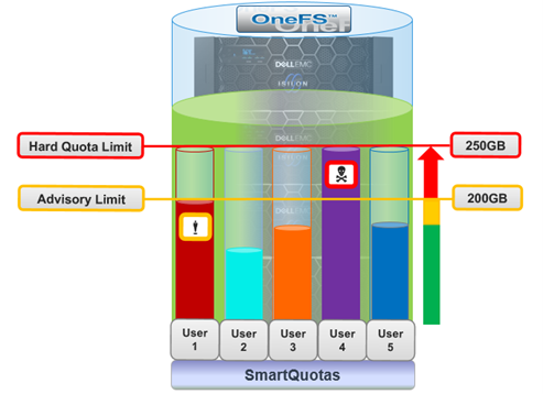
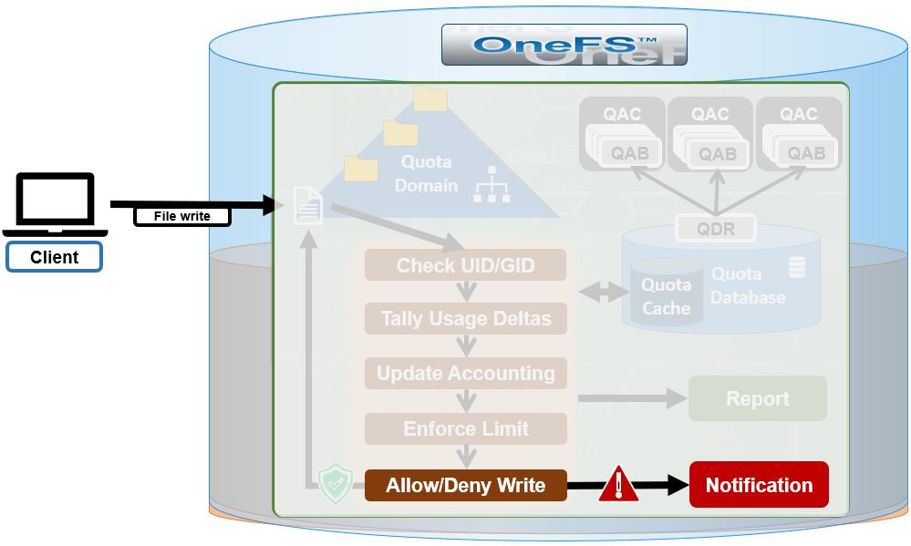
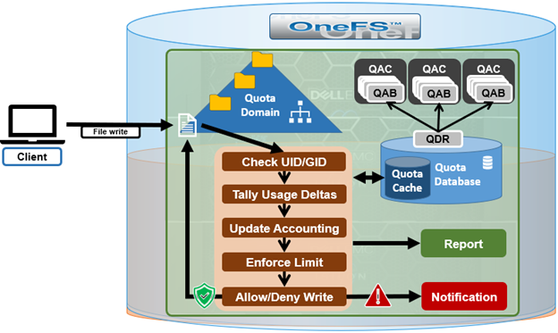
A crucial part of the OneFS SmartQuotas system is to provide user notifications regarding quota enforcement violations, both when a violation event occurs and while violation state persists on a scheduled basis.
An enforcement quota may have several notification rules associated with it. Each notification rule specifies a condition and an action to be performed when the condition is met. Notification rules are considered part of enforcements. Clearing an enforcement also clears any notification rules associated with it.
Enforcement quotas support the following notification settings:
| Quota Notification Setting | Description |
| Global default | Uses the global default notification for the specified type of quota. |
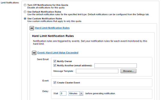
| Custom – basic | Enables creation of basic custom notifications that apply to a specific quota. Can be configured for any or all the threshold types (hard, soft, or advisory) for the specified quota. |
| Custom – advanced | Enables creation of advanced, custom notifications that apply to a specific quota. Can be configured for any or all of the threshold types (hard, soft, or advisory) for the specified quota. |
| None | Disables all notifications for the quota. |
A quota notification condition is an event which may trigger an action defined by a notification rule. These notification rules may specify a schedule (for example, “every day at 5:00 AM”) for performing an action or immediate notification of a certain condition. Examples of notification conditions include:
- Notify when a threshold is exceeded; at most, once every 5 minutes
- Notify when allocation is denied; at most, once an hour
- Notify while over threshold, daily at 2 AM
- Notify while grace period expired weekly, on Sundays at 2 AM
Notifications are triggered for events grouped by the following two categories:
| Type | Description |
| Instant notification | Includes the write-denied notification triggered when a hard threshold denies a write and the threshold-exceeded notification, triggered at the moment a hard, soft, or advisory threshold is exceeded. These are one-time notifications because they represent a discrete event in time. |
| Ongoing notification | Generated on a scheduled basis to indicate a persisting condition, such as a hard, soft, or advisory threshold being over a limit or a soft threshold’s grace period being expired for a prolonged period. |
Each notification rule can perform either one or none of the following notification actions.
| Quota Notification Action | Description |
| Alert | Sends an alert for one of the quota actions, detailed below. |
| Email Manual Address | Sends email to a specific address, or multiple addresses (OneFS 8.2 and later). |
| Email Owner | Emails an owner mapping based on its identity source. |
The email owner mapping is as follows:
| Mapping | Description |
| Active directory | Lookup is performed against the domain controller (DC). If the user does not have an email setting, a configurable transformation from user name and DC fully qualified domain name is performed in order to generate an email address. |
| LDAP | LDAP user email resolution is similar to AD users. In this case, only the email attribute looked up in the LDAP server is configurable by an administrator based on the LDAP schema for the user account information. |
| NIS | Only the configured email transformation for the NIS fully qualified domain name is used. |
| Local users | Only the configured email transformation is used. |
The actual quota notification is handled by a daemon, isi_quota_notify_d, which performs the following functions:
- Processes kernel notification events that get sent out. They are matched to notification rules to generate instant notifications (or other actions as specified in the notification rule)
- Processes notification schedules – The daemon will check notification rules on a scheduled basis. These rules specify what violation condition should trigger a notification on a regular scheduled basis.
- Performs notifications based on rule configuration to generate email messages or alert notifications.
- Manages persistent notification states so that pending events are processed in the event of a restart.
- Handles rescan requests when quotas are created or modified
SmartQuotas provides email templates for advisory, grace, and regular notification configuration, which can be found under /etc/ifs. The advisory limit email template (/etc/ifs/quota_email_advisory_template.txt) for example, displays:
Subject: Disk quota exceeded

The <ISI_QUOTA_DOMAIN_TYPE> quota on path <ISI_QUOTA_PATH> owned by <ISI_QUOTA_OWNER> has   exceeded the <ISI_QUOTA_TYPE> limit.

The quota limit is <ISI_QUOTA_THRESHOLD>, and <ISI_QUOTA_USAGE> is currently in use. <ISI_QUOTA_HARD_LIMIT> Contact your system administrator for details.
An email template contains text, and, optionally, variables that represent quota values. The following table lists the SmartQuotas variables that may be included in an email template.
| Variable | Description | Example |
| ISI_QUOTA_DOMAIN_TYPE | Quota type. Valid values are: directory, user, group, default-directory, default-user, default-group | default-directory |
| ISI_QUOTA_EXPIRATION | Expiration date of grace period | Fri Jan 8 12:34:56 PST 2021 |
| ISI_QUOTA_GRACE | Grace period, in days | 5 days |
| ISI_QUOTA_HARD_LIMIT | Includes the hard limit information of the quota to make advisory/soft email notifications more informational. | You have 30 MB left until you reach the hard quota limit of 50 MB. |
| ISI_QUOTA_NODE | Hostname of the node on which the quota event occurred | us-wa-1 |
| ISI_QUOTA_OWNER | Name of quota domain owner | jsmith |
| ISI_QUOTA_PATH | Path of quota domain | /ifs/home/jsmith |
| ISI_QUOTA_THRESHOLD | Threshold value | 20 GB |
| ISI_QUOTA_TYPE | Threshold type | Advisory |
| ISI_QUOTA_USAGE | Disk space in use | 10.5 GB |
Note that the default quota templates under /etc/ifs send are configured to send email notifications with a plain text MIME type. However, editing a template to start with an HTML tag (<html>) will allow an email client to interpret and display it as HTML content. For example:
<html><Body>

<h1>Quota Exceeded</h1><p></p>

<hr>

<p> The path <ISI_QUOTA_PATH> has exceeded the threshold <ISI_QUOTA_THRESHOLD> for this <ISI_QUOTA_TYPE> quota. </p>

</body></html>
Various system alerts are sent out to the standard cluster Alerting system when specific events occur. These include:
| Alert Type | Level | Event Description |
| NotifyFailed | Warning | An attempt to process a notification rule failed externally, such as an undelivered email. |
| NotifyConfig | Warning | A notification rule failed due to a configuration issue, such as a non-existent user or missing email address. |
| NotifyExceed | Warning | A child quota’s advisory/soft/hard limit is greater than any of parent quota’s hard limit. |
| ThresholdViolation | Info | A quota threshold was exceeded. The conditions under which this alert is triggered are defined by notification rules. |
| DomainError | Error | An invariant was violated that resulted in a forced domain rescan. |
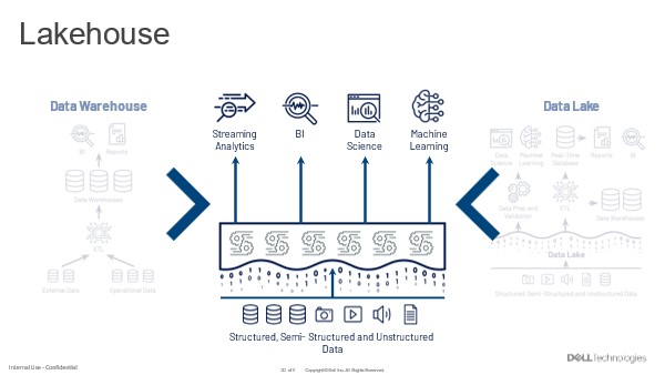
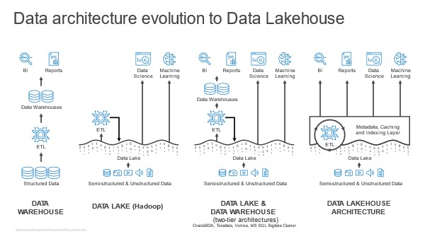
 Usually, the data lake is home to all an organization’s useful data. This data is already there. So, the data lakehouse begins with query against this data where it lives.