Author: Nick Trimbee

As we saw in the first of these blog articles, in OneFS parlance a group is a list of nodes, drives and protocols which are currently participating in the cluster. Under normal operating conditions, every node and its requisite disks are part of the current group, and the group’s status can be viewed by running sysctl efs.gmp.group on any node of the cluster.

For example, on a three node cluster:

# sysctl efs.gmp.group

efs.gmp.group: <2,288>: { 1-3:0-11, smb: 1-3, nfs: 1-3, hdfs: 1-3, all_enabled_protocols: 1-3, isi_cbind_d: 1-3, lsass: 1-3, s3: 1-3’ }

So, OneFS group info comprises three main parts:

• Sequence number: Provides identification for the group (ie.’ <2,288>’ )
• Membership list: Describes the group (ie. ‘1-3:0-11’ )
• Protocol list: Shows which nodes are supporting which protocol services (ie. { smb: 1-3, nfs: 1-3, hdfs: 1-3, all_enabled_protocols: 1-3, isi_cbind_d: 1-3, lsass: 1-3, s3: 1-3

Please note that, for the sake of ease of reading, the protocol information has been removed from each of the group strings in all the following examples.

If more detail is desired, the syscl efs.gmp.current_info command will report extensive current GMP information.

The membership list {1-3:0-11, … } represents our three node cluster, with nodes 1 through 3, each containing 12 drives, numbered zero through 11. The numbers before the colon in the group membership string represent the participating Array IDs, and the numbers after the colon are the Drive IDs.

Each node’s info is maintained in the /etc/ifs/array.xml file. For example, the entry for node 1 of the cluster above reads:

<device>

<port>5019</port>

<array_id>2</array_id>

<array_lnn>2</array_lnn>

<guid>0007430857d489899a57f2042f0b8b409a0c</guid>

<onefs_version>0x800005000100083</onefs_version>

<ondisk_onefs_version>0x800005000100083</ondisk_onefs_version>

<ipaddress name=”int-a”>192.168.76.77</ipaddress>

<status>ok</status>

<soft_fail>0</soft_fail>

<read_only>0x0</read_only>

<type>storage</type>

</device>

It’s worth noting that the Array IDs (or Node IDs as they’re also often known) differ from a cluster’s Logical Node Numbers (LNNs). LNNs are the numberings that occur within node names, as displayed by isi stat for example.

Fortunately, the isi_nodes command provides a useful cross-reference of both LNNs and Array IDs:

# isi_nodes “%{name}: LNN %{lnn}, Array ID %{id}”

node-1: LNN 1, Array ID 1

node-2: LNN 2, Array ID 2

node-3: LNN 3, Array ID 3

As a general rule, LNNs can be re-used within a cluster, whereas Array IDs are never recycled. In this case, node 1 was removed from the cluster and a new node was added instead:

node-1: LNN 1, Array ID 4

The LNN of node 1 remains the same, but its Array ID has changed to ‘4’. Regardless of how many nodes are replaced, Array IDs will never be re-used.

A node’s LNN, on the other hand, is based on the relative position of its primary backend IP address, within the allotted subnet range.

The numerals following the colon in the group membership string represent drive IDs that, like Array IDs, are also not recycled. If a drive is failed, the node will identify the replacement drive with the next unused number in sequence.

Unlike Array IDs though, Drive IDs (or Lnums, as they’re sometimes known) begin at 0 rather than at 1 and do not typically have a corresponding ‘logical’ drive number.

For example:

node-3# isi devices drive list

Lnn  Location  Device    Lnum  State   Serial

—————————————————–

3    Bay  1    /dev/da1  12    HEALTHY PN1234P9H6GPEX

3    Bay  2    /dev/da2  10    HEALTHY PN1234P9H6GL8X

3    Bay  3    /dev/da3  9     HEALTHY PN1234P9H676HX

3    Bay  4    /dev/da4  8     HEALTHY PN1234P9H66P4X

3    Bay  5    /dev/da5  7     HEALTHY PN1234P9H6GPRX

3    Bay  6    /dev/da6  6     HEALTHY PN1234P9H6DHPX

3    Bay  7    /dev/da7  5     HEALTHY PN1234P9H6DJAX

3    Bay  8    /dev/da8  4     HEALTHY PN1234P9H64MSX

3    Bay  9    /dev/da9  3     HEALTHY PN1234P9H66PEX

3    Bay 10    /dev/da10 2     HEALTHY PN1234P9H5VMPX

3    Bay 11    /dev/da11 1     HEALTHY PN1234P9H64LHX

3    Bay 12    /dev/da12 0     HEALTHY PN1234P9H66P2X

—————————————————–

Total: 12

Note that the drive in Bay 5 has an Lnum, or Drive ID, of 7, the number by which it will be represented in a group statement.

Drive bays and device names may refer to different drives at different points in time, and either could be considered a “logical” drive ID. While the best practice is definitely not to switch drives between bays of a node, if this does happen OneFS will correctly identify the relocated drives by Drive ID and thereby prevent data loss.

Depending on device availability, device names ‘/dev/da*’ may change when a node comes up, so cannot be relied upon to refer to the same device across reboots. However, Drive IDs and drive bay numbers do provide consistent drive identification.

Status info for the drives is kept in a node’s /etc/ifs/drives.xml file. Here’s the entry is for drive Lnum 0 on node Lnn 3, for example:

<logicaldrive number=”0″ seqno=”0″ active=”1″ soft-fail=”0″ ssd=”0″ purpose=”0″>66b60c9f1cd8ce1e57ad0ede0004f446</logicaldrive>

For efficiency and ease of reading, group messages combine the xml lists into a pair of numbers separated by dashes to make reporting more efficient and easier to read. For example  ‘ 1-3:0-11 ‘.

However, when a replacement disk (Lnum 12) is added to node 2, the list becomes:

{ 1:0-11, 2:0-1,3-12, 3:0-11 }.

Unfortunately, changes like these can make cluster groups trickier to read.

For example: { 1:0-23, 2:0-5,7-10,12-25, 3:0-23, 4:0-7,9-36, 5:0-35, 6:0-9,11-36 }

This describes a  cluster with two node pools. Nodes 1 to 3 contain 24 drives each, and nodes 4 through 6 are have 36 drives each. Nodes 1, 3, and 5 contain all their original drives, whereas node 2 has lost drives 6 and 11, and node 6 is missing drive 10.

Accelerator nodes are listed differently in group messages since they contain no disks to be part of the group. They’re listed twice, once as a node with no disks, and again explicitly as a ‘diskless’ node.

For example, nodes 11 and 12 in the following:

{ 1:0-23, 2,4:0-10,12-24, 5:0-10,12-16,18-25, 6:0-17,19-24, 7:0-10,12-24, 9-10:0-23, 11-12, diskless: 11-12 …}

Nodes in the process of SmartFailing are also listed both separately and in the regular group. For example, node 2 in the following:

{ 1-3:0-23, soft_failed: 2 …}

However, when the FlexProtect completes, the node will be removed from the group.

A SmartFailed node that’s also unavailable will be noted as both down and soft_failed. For example:

{ 1-3:0-23, 5:0-17,19-24, down: 4, soft_failed: 4 …}

Similarly, when a node is offline, the other nodes in the cluster will show that node as down:

{ 1-2:0-23, 4:0-23,down: 3 …}

Note that no disks for that node are listed, and that it doesn’t show up in the group.

If the node is split from the cluster—that is, if it is online but not able to contact other nodes on its back-end network—that node will see the rest of the cluster as down. Its group might look something like {6:0-11, down: 3-5,8-9,12 …} instead.

When calculating whether a cluster is below protection level, SmartFailed devices should be considered ‘in the group’ unless they are also down: a cluster with +2:1 protection with three nodes up but smartfailed does not pose an exceptional risk to data availability.

Like nodes, drives may be smartfailed and down, or smartfailed but available. The group statement looks similar to that for a smartfailed or down node, only the drive Lnum is also included. For example:

{ 1-4:0-23, 5:0-6,8-23, 6:0-17,19-24, down: 5:7, soft_failed: 5:7 }

indicates that node id 5 drive Lnum 7 is both SmartFailed and unavailable.

If the drive was SmartFailed but still available, the group would read:

{ 1-4:0-23, 5:0-6,8-23, 6:0-17,19-24, soft_failed: 5:7 }

When multiple devices are down, consolidated group statements can be tricky to read. For example, if node 1 was down, and drive 4 of node 3 was down, the group statement would read:

{ 2:0-11, 3:0-3,5-11, 4-5:0-11, down: 1, 3:4, soft_failed: 1, 3:4 }

As mentioned in the previous GMP blog article, OneFS has a read-only mode. Nodes in a read-only state are clearly marked as such in the group:

{ 1-6:0-8, soft_failed: 2, read_only: 3 }

Node 3 is listed both as a regular group member and called out separately at the end, because it’s still active. It’s worth noting that “read-only” indicates that OneFS will not write to the disks in that node. However, incoming connections to that node are still able write to other nodes in the cluster.

Non-responsive, or dead, nodes appear in groups when a node has been permanently removed from the cluster without SmartFailing the node. For example, node 11 in the following:

{ 1-5:0-11, 6:0-7,9-12, 7-10,12-14:0-11, 15:0-10,12, 16-17:0-11, dead: 11 }

Drives in a dead state include a drive number as well as a node number. For example:

{ 1:0-11, 2:0-9,11, 3:0-11, 4:0-11, 5:0-11, 6:0-11, dead: 2:10 }

In the event of a dead disk or node, the recommended course of action is to immediately start a FlexProtect and contact Isilon Support.

SmartFailed disks appear in a similar manner to other drive-specific states, and therefore include both an array ID and a drive ID. For example:

{ 1:0-11, 2:0-3,5-12, 3-4:0-11, 5:0-1,3-11, 6:0-11, soft_failed: 5:2 }

This shows drive 2 in node 5 to be SmartFailed, but still available. If the drive was physically unavailable or down, the group would show as:

{ 1:0-11, 2:0-3,5-12, 3-4:0-11, 5:0-1,3-11, 6:0-11, down: 5:2, soft_failed: 5:2 }

Stalled drives (drives that don’t respond) are marked as such, for example:

{ 1:0-2,4-11, 2-4:0-11, stalled: 1:3 }

When a drive becomes un-stalled, it simply returns to the group. In this case, the new group would return to:

{ 1-4:0-11 }

A group displays the sequence number between angle brackets. For example, <3,6>: { 1-3:0-11 }, the sequence number is <3,6>.

The first number within the sequence, in this case 3, identifies the node that initiated the most recent group change

In the case of a node leaving the group, the lowest-numbered node remaining in the cluster will initiate the group change and thus appear as the first number within the angle brackets. In the case of a node joining the group, the newly-joined node will initiate the change and thus will be the listed node. If the group change involved a single drive joining or leaving the group, the node containing that drive will initiate the change and thus will be the listed node.

The second piece of the group sequence number increases sequentially. The previous group would have had a 5 in this place; the next group should have a 7.

Rarely do we need to review sequence numbers, so long as they are increasing sequentially, and so long as they are initiated by either the lowest-numbered node, a newly-added node, or a node that removed a drive. The group membership contains the information that we most frequently require.

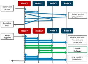
A group change occurs when an event changes devices participating in a cluster. These may be caused by drive removals or replacements, node additions, node removals, node reboots or shutdowns, backend (internal) network events, and the transition of a node into read-only mode. For debugging purposes, group change messages can be reviewed to determine whether any devices are currently in a failure state. We will explore this further in the next GMP blog article.

When a group change occurs, a cluster-wide process writes a message describing the new group membership to /var/log/messages on every node. Similarly, if a cluster “splits,” the newly-formed clusters behave in the same way: each node records its group membership to /var/log/messages. When a cluster splits, it breaks into multiple clusters (multiple groups). This is rarely, if ever, a desirable event. Notice that cluster and group are synonymous: a cluster is defined by its group members. Group members which lose sight of other group members no longer belong to the same group and thus no longer belong to the same cluster.

To view group changes from one node’s perspective, you can grep for the expression ‘new group’ to extract the group change statements from the log. For example:

tme-1# grep -i ‘new group’ /var/log/messages | tail –n 10

Nov 8 08:07:50 (id1) /boot/kernel/kernel: [gmp_info.c:530](pid 1814=”kt: gmpdrive-upda”) new group: : { 1:0-4, down: 1:5-11, 2-3 }

Nov 8 08:07:50 (id1) /boot/kernel/kernel: [gmp_info.c:530](pid 1814=”kt: gmpdrive-upda”) new group: : { 1:0-5, down: 1:6-11, 2-3 }

Nov 8 08:07:50 (id1) /boot/kernel/kernel: [gmp_info.c:530](pid 1814=”kt: gmpdrive-upda”) new group: : { 1:0-6, down: 1:7-11, 2-3 }

Nov 8 08:07:50 (id1) /boot/kernel/kernel: [gmp_info.c:530](pid 1814=”kt: gmpdrive-upda”) new group: : { 1:0-7, down: 1:8-11, 2-3 }

Nov 8 08:07:50 (id1) /boot/kernel/kernel: [gmp_info.c:530](pid 1814=”kt: gmpdrive-upda”) new group: : { 1:0-8, down: 1:9-11, 2-3 }

Nov 8 08:07:50 (id1) /boot/kernel/kernel: [gmp_info.c:530](pid 1814=”kt: gmpdrive-upda”) new group: : { 1:0-9, down: 1:10-11, 2-3 }

Nov 8 08:07:50 (id1) /boot/kernel/kernel: [gmp_info.c:530](pid 1814=”kt: gmpdrive-upda”) new group: : { 1:0-10, down: 1:11, 2-3 }

Nov 8 08:07:50 (id1) /boot/kernel/kernel: [gmp_info.c:530](pid 1814=”kt: gmpdrive-upda”) new group: : { 1:0-11, down: 2-3 }

Nov 8 08:07:51 (id1) /boot/kernel/kernel: [gmp_info.c:530](pid 1814=”kt: gmpmerge”) new group: : { 1:0-11, 3:0-7,9-12, down: 2 }

Nov 8 08:07:52 (id1) /boot/kernel/kernel: [gmp_info.c:530](pid 1814=”kt: gmpmerge”) new group: : {

In this case, the tail -10 command has been used to limit the returned group changes to the last ten reported in the file. All of these occur within two seconds, so in the case of an actual case, we would want to go further back, to before whatever incident was under investigation.

INTERPRETING GROUP CHANGES

Even in the example above, however, we can be sure of several things:

• Most importantly, at last report all nodes of the cluster are operational and joined into the cluster. No nodes or drives report as down or split. (At some point in the past, drive ID 8 on node 3 was replaced, but a replacement disk has been added successfully.)
• Next most important is that node 1 rebooted: for the first eight out of ten lines, each group change is adding back a drive on node 1 into the group, and nodes two and three are inaccessible. This occurs on node reboot prior to any attempt to join an active group and is correct and healthy behavior.
• Note also that node 3 joins in with node 1 before node 2 does. This might be coincidental, given that the two nodes join within a second of each other. On the other hand, perhaps node 2 also rebooted while node 3 remained up. A review of group changes from these other nodes could confirm either of those behaviors.

Logging onto node 3, we can see the following:

tme-1# grep -i ‘new group’ /var/log/messages | tail -10

Jul 8 08:07:50 (id3) /boot/kernel/kernel: [gmp_info.c:530](pid 1828=”kt: gmpdrive-upda”) new group: : { 3:0-4, down: 1-2, 3:5-7,9-12 }

Jul 8 08:07:50 (id3) /boot/kernel/kernel: [gmp_info.c:530](pid 1828=”kt: gmpdrive-upda”) new group: : { 3:0-5, down: 1-2, 3:6-7,9-12 }

Jul 8 08:07:50 (id3) /boot/kernel/kernel: [gmp_info.c:530](pid 1828=”kt: gmpdrive-upda”) new group: : { 3:0-6, down: 1-2, 3:7,9-12 }

Jul 8 08:07:50 (id3) /boot/kernel/kernel: [gmp_info.c:530](pid 1828=”kt: gmpdrive-upda”) new group: : { 3:0-7, down: 1-2, 3:9-12 }

Jul 8 08:07:50 (id3) /boot/kernel/kernel: [gmp_info.c:530](pid 1828=”kt: gmpdrive-upda”) new group: : { 3:0-7,9, down: 1-2, 3:10-12 }

Jul 8 08:07:50 (id3) /boot/kernel/kernel: [gmp_info.c:530](pid 1828=”kt: gmpdrive-upda”) new group: : { 3:0-7,9-10, down: 1-2, 3:11-12 }

Jul 8 08:07:50 (id3) /boot/kernel/kernel: [gmp_info.c:530](pid 1828=”kt: gmpdrive-upda”) new group: : { 3:0-7,9-11, down: 1-2, 3:12 }

Jul 8 08:07:50 (id3) /boot/kernel/kernel: [gmp_info.c:530](pid 1828=”kt: gmpdrive-upda”) new group: : { 3:0-7,9-12, down: 1-2 }

Jul 8 08:07:50 (id3) /boot/kernel/kernel: [gmp_info.c:530](pid 1828=”kt: gmpmerge”) new group: : { 1:0-11, 3:0-7,9-12, down: 2 }

Jul 8 08:07:52 (id3) /boot/kernel/kernel: [gmp_info.c:530](pid 1828=”kt: gmpmerge”) new group: : { 1-2:0-11, 3:0-7,9-12 }

In this instance, it’s apparent that node 3 rebooted at the same time. It’s worth checking node 2’s logs to see if it also rebooted at the same time.

Given that all three nodes rebooted simultaneously, it’s highly likely that this was a cluster-wide event, rather than a single-node issue – especially since watchdog timeouts that cause cluster-wide reboots typically cause staggered rather than simultaneous reboots. The Softwatch process (also known as software watchdog or swatchdog) monitors the kernel and dumps a stack trace and/or reboots the node when the node is not responding. This tool protects the cluster from the impact of heavy CPU starvation and aids issue discovery and resolution process.

Constructing a timeline

If a cluster experiences multiple, staggered group changes, it can be extremely helpful to craft a timeline of the order and duration in which nodes are up or down. This timeline illustrates with. This info can be cross-referenced with panic stack traces and other system logs to help diagnose the root cause of an event.

For example, in the following a 15-node cluster experiences six different node reboots over a twenty-minute period. These are the group change messages from node 14, which that stayed up the whole duration:

tme-14# grep ‘new group’ tme-14-messages

Jul 8 16:44:38 tme-14(id20) /boot/kernel/kernel: [gmp_info.c:510](pid 1060=”kt: gmp-split”) new group: : { 1-2:0-11, 6-8, 13-15:0-11, 16:0,2-12, 17- 18:0-11, 19-21, down: 9}

Jul 8 16:44:58 tme-14(id20) /boot/kernel/kernel: [gmp_info.c:510](pid 1066=”kt: gmp-split”) new group: : { 1:0-11, 6-8, 13-14:0-11, 16:0,2-12, 17- 18:0-11, 19-21, down: 2, 9, 15}

Jul 8 16:45:20 tme-14(id20) /boot/kernel/kernel: [gmp_info.c:510](pid 1066=”kt: gmp-split”) new group: : { 1:0-11, 6-8, 14:0-11, 16:0,2-12, 17-18:0- 11, 19-21, down: 2, 9, 13, 15} Mar 26 16:47:09 tme-14(id20) /boot/kernel/kernel: [gmp_info.c:510](pid 1066=”kt: gmp-merge”) new group: : { 1:0-11, 6-8, 9,14:0-11, 16:0,2-12, 17- 18:0-11, 19-21, down: 2, 13, 15}

Jul 8 16:47:27 tme-14(id20) /boot/kernel/kernel: [gmp_info.c:510](pid 1066=”kt: gmp-split”) new group: : { 6-8, 9,14:0-11, 16:0,2-12, 17-18:0-11, 19-21, down: 1-2, 13, 15}

Jul 8 16:48:11 tme-14(id20) /boot/kernel/kernel: [gmp_info.c:510](pid 2102=”kt: gmp-split”) new group: : { 6-8, 9,14:0-11, 16:0,2-12, 17:0-11, 19- 21, down: 1-2, 13, 15, 18}

Jul 8 16:50:55 tme-14(id20) /boot/kernel/kernel: [gmp_info.c:510](pid 2102=”kt: gmp-merge”) new group: : { 6-8, 9,13-14:0-11, 16:0,2-12, 17:0-11, 19- 21, down: 1-2, 15, 18}

Jul 8 16:51:26 tme-14(id20) /boot/kernel/kernel: [gmp_info.c:510](pid 85396=”kt: gmp-merge”) new group: : { 2:0-11, 6-8, 9,13-14:0-11, 16:0,2-12, 17:0-11, 19-21, down: 1, 15, 18}

Jul 8 16:51:53 tme-14(id20) /boot/kernel/kernel: [gmp_info.c:510](pid 85396=”kt: gmp-merge”) new group: : { 2:0-11, 6-8, 9,13-15:0-11, 16:0,2-12, 17:0-11, 19-21, down: 1, 18}

Jul 8 16:54:06 tme-14(id20) /boot/kernel/kernel: [gmp_info.c:510](pid 85396=”kt: gmp-merge”) new group: : { 1-2:0-11, 6-8, 9,13-15:0-11, 16:0,2-12, 17:0-11, 19-21, down: 18}

Jul 8 16:56:10 tme-14(id20) /boot/kernel/kernel: [gmp_info.c:510](pid 2102=”kt: gmp-merge”) new group: : { 1-2:0-11, 6-8, 9,13-15:0-11, 16:0,2-12, 17-18:0-11, 19-21}

Jul 8 16:59:54 tme-14(id20) /boot/kernel/kernel: [gmp_info.c:510](pid 85396=”kt: gmp-split”) new group: : { 1-2:0-11, 6-8, 9,13-15,17-18:0-11, 19-21, down: 16}

Jul 8 17:05:23 tme-14(id20) /boot/kernel/kernel: [gmp_info.c:510](pid 1066=”kt: gmp-merge”) new group: : { 1-2:0-11, 6-8, 9,13-15:0-11, 16:0,2-12, 17-18:0-11, 19-21}

First, run the isi_nodes “%{name}: LNN %{lnn}, Array ID %{id}” to map the cluster’s node names to their respective Array IDs.

Before the cluster node outage event on Jul 8, we can see there was a group change on Jul 3

Jul 8 14:54:00 tme-14(id20) /boot/kernel/kernel: [gmp_info.c:510](pid 1060=”kt: gmp-merge”) new group: : { 1-2:0-11, 6-8, 9,13-15:0-11, 16:0,2-12, 17-18:0-11, 19-21, diskless: 6-8, 19-21 }

After that, all nodes came back online, and the cluster could be considered healthy. The cluster contains six accelerators, and all nine data nodes with twelve drives apiece. Since the Array IDs now extend to 21, and Array IDs 3 through 5 and 10 through 12 are missing, this confirms that six nodes were added or removed from the cluster.

So, the first event occurs at 16:44:38 on 8 July:

Jul 8 16:44:38 tme-14(id20) /boot/kernel/kernel: [gmp_info.c:510](pid 1060=”kt: gmp-split”) new group: : { 1-2:0-11, 6-8, 13-15:0-11, 16:0,2-12, 17- 18:0-11, 19-21, down: 9, diskless: 6-8, 19-21 }

Node 14 identifies Array ID 9 (LNN 6) as having left the group.

Next, twenty seconds later, two more nodes (2 & 15) show as offline:

Jul 8 16:44:58 tme-14(id20) /boot/kernel/kernel: [gmp_info.c:510](pid 1066=”kt: gmp-split”) new group: : { 1:0-11, 6-8, 13-14:0-11, 16:0,2-12, 17- 18:0-11, 19-21, down: 2, 9, 15, diskless: 6-8, 19-21 }

Twenty-two seconds later, another node goes offline:

Jul 8 16:45:20 tme-14(id20) /boot/kernel/kernel: [gmp_info.c:510](pid 1066=”kt: gmp-split”) new group: : { 1:0-11, 6-8, 14:0-11, 16:0,2-12, 17-18:0- 11, 19-21, down: 2, 9, 13, 15, diskless: 6-8, 19-21 }

At this point, four nodes (2,6,7, & 9) are marked as being offline:

Nearly two minutes later, the previously down node (node 6) rejoins:

Jul 8 16:47:09 tme-14(id20) /boot/kernel/kernel: [gmp_info.c:510](pid 1066=”kt: gmp-merge”) new group: : { 1:0-11, 6-8, 9,14:0-11, 16:0,2-12, 17- 18:0-11, 19-21, down: 2, 13, 15, diskless: 6-8, 19-21 }

Twenty-five seconds after node 6 comes back, however, node 1 goes offline:

Jul 8 16:47:27 tme-14(id20) /boot/kernel/kernel: [gmp_info.c:510](pid 1066=”kt: gmp-split”) new group: : { 6-8, 9,14:0-11, 16:0,2-12, 17-18:0-11, 19-21, down: 1-2, 13, 15, diskless: 6-8, 19-21 }

Finally, the group returns to the same as the original group:

Jul 8 17:05:23 tme-14(id20) /boot/kernel/kernel: [gmp_info.c:510](pid 1066=”kt: gmp-merge”) new group: : { 1-2:0-11, 6-8, 9,13-15:0-11, 16:0,2-12, 17-18:0-11, 19-21, diskless: 6-8, 19-21 }

As such, a timeline of this cluster event could read:

Jul 8 16:44:38 6 down

Jul 8 16:44:58 2, 9 down (6 still down)

Jul 8 16:45:20 7 down (2, 6, 9 still down)

Jul 8 16:47:09 6 up (2, 7, 9 still down)

Jul 8 16:47:27 1 down (2, 7, 9 still down)

Jul 8 16:48:11 12 down (1, 2, 7, 9 still down)

Jul 8 16:50:55 7 up (1, 2, 9, 12 still down)

Jul 8 16:51:26 2 up (1, 9, 12 still down)

Jul 8 16:51:53 9 up (1, 12 still down)

Jul 8 16:54:06 1 up (12 still down)

Jul 8 16:56:10 12 up (none down)

Jul 8 16:59:54 10 down

Jul 8 17:05:23 10 up (none down)

Before triangulating log events across multiple nodes, it’s important to ensure that the nodes’ clocks are all synchronized. To check this, run the isi_for_array –q date command on all nodes and confirm that they match. If not, apply the time offset for a particular node to the timestamps of its logfiles.

So what caused node 6 to go offline at 16:44:38? The messages file for that node show that nothing of note occurred between noon on Jul 8 and 16:44:31. After this, a slew of messages were logged:

Jul 8 16:44:31 tme-tme-6(id9) /boot/kernel/kernel: [rbm_device.c:749](pid 132=”swi5: clock sio”) ping failure (1)

Jul 8 16:44:31 tme-tme-6(id9) /boot/kernel/kernel: last 3 messages out: GMP_NODE_INFO_UPDATE, GMP_NODE_INFO_UPDATE, LOCK_REQ

Jul 8 16:44:31 tme-tme-6(id9) /boot/kernel/kernel: last 3 messages in : LOCK_RESP, TXN_COMMITTED, TXN_PREPARED

These three messages are repeated several times and then node 6 splits:

Jul 8 16:44:31 tme-tme-6(id9) /boot/kernel/kernel: [rbm_device.c:749](pid 132=”swi5: clock sio”) ping failure (21)

Jul 8 16:44:31 tme-tme-6(id9) /boot/kernel/kernel: last 3 messages out: GMP_NODE_INFO_UPDATE, GMP_NODE_INFO_UPDATE, LOCK_RESP

Jul 8 16:44:31 tme-6(id9) /boot/kernel/kernel: last 3 messages in : LOCK_REQ, LOCK_RESP, LOCK_RESP

Jul 8 16:44:34 tme-6(id9) /boot/kernel/kernel: [gmp_info.c:650](pid 48538=”kt: disco-cbs”) disconnected from node 1

Jul 8 16:44:34 tme-6(id9) /boot/kernel/kernel: [gmp_info.c:650](pid 49215=”kt: disco-cbs”) disconnected from node 2

Jul 8 16:44:34 tme-6(id9) /boot/kernel/kernel: [gmp_info.c:650](pid 50864=”kt: disco-cbs”) disconnected from node 6

Jul 8 16:44:34 tme-6(id9) /boot/kernel/kernel: [gmp_info.c:650](pid 49114=”kt: disco-cbs”) disconnected from node 7

Jul 8 16:44:34 tme-6(id9) /boot/kernel/kernel: [gmp_info.c:650](pid 30433=”kt: disco-cbs”) disconnected from node 8

Jul 8 16:44:34 tme-6(id9) /boot/kernel/kernel: [gmp_info.c:650](pid 49218=”kt: disco-cbs”) disconnected from node 13

Jul 8 16:44:34 tme-6(id9) /boot/kernel/kernel: [gmp_info.c:650](pid 50903=”kt: disco-cbs”) disconnected from node 14

Jul 8 16:44:34 tme-6(id9) /boot/kernel/kernel: [gmp_info.c:650](pid 24705=”kt: disco-cbs”) disconnected from node 15

Jul 8 16:44:34 tme-6(id9) /boot/kernel/kernel: [gmp_info.c:650](pid 48574=”kt: disco-cbs”) disconnected from node 16

Jul 8 16:44:34 tme-6(id9) /boot/kernel/kernel: [gmp_info.c:650](pid 49508=”kt: disco-cbs”) disconnected from node 17

Jul 8 16:44:34 tme-6(id9) /boot/kernel/kernel: [gmp_info.c:650](pid 52977=”kt: disco-cbs”) disconnected from node 18

Jul 8 16:44:34 tme-6(id9) /boot/kernel/kernel: [gmp_info.c:650](pid 52975=”kt: disco-cbs”) disconnected from node 19

Jul 8 16:44:34 tme-6(id9) /boot/kernel/kernel: [gmp_info.c:650](pid 50902=”kt: disco-cbs”) disconnected from node 20

Jul 8 16:44:34 tme-6(id9) /boot/kernel/kernel: [gmp_info.c:650](pid 48513=”kt: disco-cbs”) disconnected from node 21

Jul 8 16:44:34 tme-6(id9) /boot/kernel/kernel: [gmp_rtxn.c:194](pid 48513=”kt: gmp-split”) forcing disconnects from { 1, 2, 6, 7, 8, 13, 14, 15, 16, 17, 18, 19, 20, 21 }

Jul 8 16:44:50 tme-6(id9) /boot/kernel/kernel: [gmp_info.c:510](pid 48513=”kt: gmp-split”) new group: : { 9:0-11, down: 1-2, 6-8, 13-21, diskless: 6-8, 19-21 }

Node 6 splits from the rest of the nodes, then rejoins the rest of the cluster without a reboot.

Review messages logs for other nodes

After grabbing the pertinent node state and event info from the /var/log/messages logs for all fifteen nodes, a final timeline could read:

Jul 8 16:44:38 6 down

6: *** – split, not rebooted. Network issue? No engine stalls1 at that time…

Jul 8 16:44:58 2, 9 down (6 still down)

2: Softwatch timed out

9: Softwatch timed out

Jul 8 16:45:20 7 down (2, 6, 9 still down)

7: Indeterminate transactions

Jul 8 16:47:09 6 up (2, 7, 9 still down)

Jul 8 16:47:27 1 down (2, 7, 9 still down)

1: Softwatch timed out

Jul 8 16:48:11 12 down (1, 2, 7, 9 still down)

12: Softwatch timed out

Jul 8 16:50:55 7 up (1, 2, 9, 12 still down)

Jul 8 16:51:26 2 up (1, 9, 12 still down)

Jul 8 16:51:53 9 up (1, 12 still down)

Jul 8 16:54:06 1 up (12 still down)

Jul 8 16:56:10 12 up (none down)

Jul 8 16:59:54 10 down

10: Indeterminate transactions

Jul 8 17:05:23 10 up (none down)

Note: The BAM (block allocation manager) is responsible for building and executing a ‘write plan’ of which blocks should be written to which drives on which nodes for each transaction. OneFS logs an engine stall if this write plan encounters an unexpected delay.

Because group changes document the cluster’s actual configuration from OneFS’ perspective, they’re a vital tool in understanding at any point in time which devices the cluster considers available, and which devices the cluster considers as having failed. This info, when combined with other data from cluster logs, can provide a succinct but detailed cluster history, simplifying both debugging and failure analysis.

By popular request, we’ll explore the topic of cluster state changes and quorum over the next couple of blog articles .

In computer science, Brewer’s CAP theorem states that it’s impossible for a distributed system to simultaneously guarantee consistency, availability, and partition tolerance. This means that, when faced with a network partition, one has to choose between consistency and availability.

OneFS does not compromise on consistency, so a mechanism is required to manage a cluster’s transient state and quorum.  As such, the primary role of the OneFS Group Management Protocol (GMP) is to help create and maintain a group of synchronized nodes. Having a consistent view of the cluster state is critical, since initiators need to know which node and drives are available to write to, etc. A group is a given set of nodes which have synchronized state, and a cluster may form multiple groups as connection state changes. GMP distributes a variety of state information about nodes and drives, from identifiers to usage statistics. The most fundamental of these is the composition of the cluster, or ‘static aspect’ of the group, which is stored in the array.xml file. The array.xml file also includes info such as the ID, GUID, and whether the node is diskless or storage, plus attributes not considered part of the static aspect, such as internal IP addresses.

Similarly, the state of a node’s drives is stored in the drives.xml file, along with a flag indicating whether the drive is an SSD. Whereas GMP manages node states directly, drive states are actually managed by the ‘drv’ module, and broadcast via GMP. A significant difference between nodes and drives is that for nodes, the static aspect is distributed to every node in the array.xml file, whereas drive state is only stored locally on a node. The array.xml information is needed by every node in order to define the cluster and allow nodes to form connections. In contrast, drives.xml is only stored locally on a node. When a node goes down, other nodes have no method to obtain the drive configuration of that node. Drive information may be cached by the GMP, but it is not available if that cache is cleared.

Conversely, ‘dynamic aspect’ refers to the state of nodes and drives which may change. These states indicate the health of nodes and their drives to the various file system modules – plus whether or not components can be used for particular operations. For example, a soft-failed node or drive should not be used for new allocations. These components can be in one of seven states:

• UP The component is responding.
• DOWN The component is not responding.
• DEAD The component is not allowed to come back to the UP state and should be removed.
• STALLED A drive is responding slowly.
• GONE The component has been removed.
• Soft-failed The component is in the process of being removed.
• Read-only This state only applies to nodes.

Note: A node or drive may go from ‘down, soft-failed’ to ‘up, soft-failed’ and back. These flags are persistently stored in the array.xml file for nodes and the drives.xml file for drives.

Group and drive state information allows the various file system modules to make timely and accurate decisions about how they should utilize nodes and drives. For example, when reading a block, the selected mirror should be on a node and drive where a read can succeed (if possible). File system modules use the GMP to test for node and drive capabilities, which include:

• Readable                 Drives on this node may be read.
• Writable                  Drives on this node may be written to.
• Restripe From      Move blocks away from the node.

Access levels help define ‘as a last resort’ with states for which access should be avoided unless necessary. The access levels, in order of increased access, are as follows:

• Normal                     The default access level.
• Read Stalled           Allows reading from stalled drives.
• Modify Stalled      Allows writing to stalled drives.
• Read Soft-fail       Allows reading from soft-failed nodes and drives.
• Never                        Indicates a group state never supports the capability.

Drive state and node state capabilities are shown in the following tables. As shown, the only group states affected by increasing access levels are soft-failed and stalled.

 Minimum Access Level for Capabilities Per Node State

Minimum Access Level for Capabilities Per Drive State

OneFS depends on a consistent view of a cluster’s group state. For example, some decisions, such as choosing lock coordinators, are made assuming all nodes have the same coherent notion of the cluster.

Group changes originate from multiple sources, depending on the particular state. Drive group changes are initiated by the drv module. Service group changes are initiated by processes opening and closing service devices. Each group change creates a new group ID, comprising a node ID and a group serial number. This group ID can be used to quickly determine whether a cluster’s group has changed, and is invaluable for troubleshooting cluster issues, by identifying the history of group changes across the nodes’ log files.

GMP provides coherent cluster state transitions using a process similar to two-phase commit, with the up and down states for nodes being directly managed by the GMP. RBM or Remote Block Manager code provides the communication channel that connect devices in the OneFS. When a node mounts /ifs it initializes the RBM in order to connect to the other nodes in the cluster, and uses it to exchange GMP Info, negotiate locks, and access data on the other nodes.

Before /ifs is mounted, a ‘cluster’ is just a list of MAC and IP addresses in array.xml, managed by ibootd when nodes join or leave the cluster. When mount_efs is called, it must first determine what it‘s contributing to the file system, based on the information in drives.xml. After a cluster (re)boot, the first node to mount /ifs is immediately placed into a group on its own, with all other nodes marked down. As the Remote Block Manager (RBM) forms connections, the GMP merges the connected nodes, enlarging the group until the full cluster is represented. Group transactions where nodes transition to UP are called a ‘merge’, whereas a node transitioning to down is called a split. Several file system modules must update internal state to accommodate splits and merges of nodes. Primarily, this is related to synchronizing memory state between nodes.

The soft-failed, read-only, and dead states are not directly managed by the GMP. These states are persistent and must be written to array.xml accordingly. Soft-failed state changes are often initiated from the user interface, for example via the ‘isi devices’ command.

A GMP group relies on cluster quorum to enforce consistency across node disconnects. By requiring ⌊N/2⌋+1 replicas to be available, this ensures that no updates are lost. Since nodes and drives in OneFS may be readable, but not writable, OneFS has two quorum properties:

• Read quorum
• Write quorum

Read quorum is governed by having [N/2] + 1 nodes readable, as indicated by sysctl efs.gmp.has_quorum. Similarly, write quorum requires at least [N/2] + 1 writeable nodes, as represented by the sysctl efs.gmp.has_super_block_quorum. A group of nodes with quorum is called the ‘majority’ side, whereas a group without quorum is a ‘minority’. By definition, there can only be one ‘majority’ group, but there may be multiple ‘minority’ groups. A group which has any components in any state other than up is referred to as degraded.

File system operations typically query a GMP group several times before completing. A group may change over the course of an operation, but the operation needs a consistent view. This is provided by the group info, which is the primary interface modules use to query group state. The current group info can be viewed via the sysctl efs.gmp.current_info command. It includes the GMP’s group state, but also information about services provided by nodes in the cluster. This allows nodes in the cluster to discover when services change state on other nodes and take the appropriate action when this happens. An example is SMB lock expiry, which uses GMP service information to clean up locks held by other nodes when the service owning the lock goes down.

Processes change the service state in GMP by opening and closing service devices. A particular service will transition from down to up in the GMP group when it opens the file descriptor for a device. Closing the service file descriptor will trigger a group change that reports the service as down. A process can explicitly close the file descriptor if it chooses, but most often the file descriptor will remain open for the duration of the process and closed automatically by the kernel when it terminates.

An understanding of OneFS groups and their related group change messages allows you to determine the current health of a cluster – as well as reconstruct the cluster’s history when troubleshooting issues that involve cluster stability, network health, and data integrity. We’ll explore the reading and interpretation of group change status data in the second part of this blog article series.

First introduced in version 9.0, OneFS provides support for IPMI, the Intelligent Platform Management Interface protocol. IPMI allows out-of-band console access and remote power control across a dedicated ethernet interface via Serial over LAN (SoL). As such, IMPI provides true lights-out management for PowerScale F-series all-flash nodes and Gen6 H-series and A-series chassis without the need for additional rs-232 serial port concentrators or PDU rack power controllers.

For example, IPMI enables individual nodes or the entire cluster to be powered on after maintenance or a power outage. For example:

• Power off nodes or the cluster, such as after a power outage and when the cluster is operating on backup power.
• Perform a Hard/Cold Reboot/Power Cycle, for example, if a node is unresponsive to OneFS.

IPMI is disabled by default in OneFS 9.0 and later, but can be easily enabled, configured, and operated from the CLI via the new ‘isi ipmi’ command set.

A cluster’s console can easily be accessed using the IPMItool utility, available as part of most Linux distributions, or accessible through other proprietary tools. For the PowerScale F900, F600 and F200 platforms, the Dell iDRAC remote console option can be accessed via an https web browser session to the default port 443 at a node’s IPMI address.

Note that support for IPMI on Isilon Generation 6 hardware requires node firmware package 10.3.2 and SSP firmware 02.81 or later.

With OneFS 9.0 and later, IPMI is fully supported on both PowerScale Gen6 H-series and A-series chassis-based platforms, and PowerScale all-flash F-series platforms. For Gen6 nodes running 8.2.x releases, IPMI is not officially supported but does generally work.

IPMI can be configured for DHCP, static IP, or a range of IP addresses. With the range option, IP addresses are allocated on a first-available basis and be cannot assign a specific IP address to a specific node. For security purposes, the recommendation is to restrict IPMI traffic to a dedicated, management-only VLAN.

A single username and password is configured for IPMI management across all the nodes in a cluster using isi ipmi user modify — username= –set-password CLI syntax. Usernames can be up to 16 characters in length, and passwords must comprise 17-20 characters. To verify the username configuration, use isi ipmi user view.

Be aware that a node’s physical serial port is disabled when a SoL session is active, but becomes re-enabled when the SoL session is terminated with the ‘deactivate’ command option.

In order to run the OneFS IPMI commands, the administrative account being used must have the RBAC ISI_PRIV_IPMI privilege.

The following CLI syntax can be used to enable IPMI for DHCP:

# isi ipmi settings modify --enabled=True --allocation-type=dhcp 35 426 IPMI

Simiarly, to enable IPMI for a static IP address:

# isi ipmi settings modify --enabled=True --allocation-type=static

To enable IPMI for a range of IP addresses use:

# isi ipmi network modify --gateway=[gateway IP] --prefixlen= --ranges=[IP Range]

The power control and Serial over LAN features can be configured and viewed using the following CLI command syntax. For example:

# isi ipmi features list

ID            Feature Description           Enabled
----------------------------------------------------
Power-Control Remote power control commands Yes

SOL           Serial over Lan functionality Yes
----------------------------------------------------

To enable the power control feature:

# isi ipmi features modify Power-Control --enabled=True

To enable the Serial over LAN (SoL) feature:

# isi ipmi features modify SOL --enabled=True

The following CLI commands can be used to configure a single username and password to perform IPMI tasks across all nodes in a cluster. Note that usernames can be up to 16 characters in length, while the associated passwords must be 17-20 characters in length.

To configure the username and password, run the CLI command:

# isi ipmi user modify --username [Username] --set-password

To confirm the username configuration, use:

# isi ipmi user view

Username: power

In this case, the user ‘power’ has been configured for OneFS IPMI control.

On the client side, the ‘ipmiItool’ command utility is ubiquitous in the Linux and UNIX world, and is included natively as part of most distributions. If not, it can easily be installed using the appropriate package manager, such as ‘yum’.

The ipmitool usage syntax is as follows:

[Linux Host:~]$ ipmitool -I lanplus -H [Node IP] -U [Username] -L OPERATOR -P [password]

For example, to execute power control commands:

ipmitool -I lanplus -H [Node IP] -U [Username] -L OPERATOR -P [password] power [command]

The ‘power’ command options above include status, on, off, cycle, and reset.

And, similarly, for Serial over LAN:

ipmitool -I lanplus -H [Node IP] -U [Username] -L OPERATOR -P [password] sol [command]

The serial over LAN ‘command’ options include info, activate, and deactivate.

Once active, a Serial over LAN session can easily be exited using the ‘tilde dot’ command syntax, as follows:

# ~.

On PowerScale F600 and F200 nodes, the remote console can be accessed via the Dell iDRAC by browsing to https://<node_IPMI_IP_address>:443 and, unless it’s been changed, using the default password of root/calvin.

Double clicking on the ‘Virtual Console’ image on the bottom right of the iDRAC main page above brings up a full-size console window:

From here, authenticate using your preferred cluster username and password for full out-of-band access to the OneFS console.

When it comes to troubleshooting OneFS IPMI, a good place to start is by checking that the daemon is enabled. This can be done using the following CLI command:

# isi services -a | grep -i ipmi_mgmt

isi_ipmi_mgmt_d      Manages remote IPMI configuration        EnabledTroubleshooting & Firmware

The IPMI management daemon, isi_ipmi_mgmt_d, can also be run with a variety of options including the -s flag to list the current IPMI settings across the cluster, the -d flag to enable debugging output, etc, as follows:

# /usr/bin/isi_ipmi_mgmt_d -h

usage: isi_ipmi_mgmt_d [-h] [-d] [-m] [-s] [-c CONFIG]

Daemon that manages the remote IPMI configuration.

optional arguments:

-h, --help            show this help message and exit

-d, --debug           Enable debug logging

-m, --monitor         Launch the remote IPMI monitor daemon

-s, --show            Show the remote IPMI settings

-c CONFIG, --config CONFIG

Configure IPMI management settings

IPMI writes errors, warnings, etc, to its log file, located at /var/log/isi_ipmi_mgmt_d.log, and which includes a host of useful troubleshooting information.

First introduced in version 9.0,  OneFS supports the AWS S3 API as a protocol, extending the PowerScale data lake to natively include object, and enabling workloads which write data via file protocols such as NFS, HDFS or SMB, and then read that data via S3, or vice versa.

Because objects are files “under the hood”, the same OneFS data services, such as Snapshots, SyncIQ, WORM, etc, are all seamlessly integrated.

Applications now have multiple access options – across both file and object – to the same underlying dataset, semantics, and services, eliminating the need for replication or migration for different access requirements, and vastly simplifying management.

This makes it possible to run hybrid and cloud-native workloads, which use S3-compatible backend storage, for example cloud backup & archive software, modern apps, analytics flows, IoT workloads, etc. – and to run these on-prem, alongside and coexisting with traditional file-based workflows.

In addition to HTTP 1.1, OneFS S3 supports HTTPS 1.2, to meet organizations’ security and compliance needs. And since S3 is integrated as a top-tier protocol, performance is anticipated to be similar to SMB.

By default, the S3 service listens on port 9020 for HTTP and 9021 for HTTPS, although both these ports are easily configurable.

Every S3 object is linked to a file, and each S3 bucket maps to a specific directory called the bucket path.  If the bucket path is not specified, a default is used. When creating a bucket, OneFS adds a dot-s3 directory under the bucket path, which is used to store temporary files for PUT objects.

The AWS S3 data model is a flat structure, without a strict hierarchy of sub-buckets or sub-folders. However, it does provide a logical hierarchy, using object key-name prefixes and delimiters, which OneFS leverages to support a rudimentary concept of folders.

OneFS S3 also incorporates multi-part upload, using HTTP’s ‘100 continue’ header, allowing OneFS to ingest large objects, or copy existing objects, in parts, thereby improving upload performance.

OneFS allows both ‘virtual hosted-style requests’, where you specify a bucket in a request using the HTTP Host header, and also ‘path-style requests’, where a bucket is specified using the first slash-delimited component of the Request-URI path.

Every interaction with S3 is either authenticated or anonymous. While authentication verifies the identity of the requester, authorization controls access to the desired data. OneFS treats unauthenticated requests as anonymous, mapping it to the user ‘nobody’.

OneFS S3 uses either AWS Signature Version 2 or Version 4 to authenticate requests, which must include a signature value that authenticates the request sender. This requires the user to have both an access ID and a secret Key, which can be obtained from the OneFS key management portal.

The secret key is used to generate the signature value, along with several request header values. After receiving the signed request, OneFS uses the access ID to retrieve a copy of the secret key internally, recomputes the signature value of the request, and compares it against the received signature. If they match, the requester is authenticated, and any header value used in the signature is verified to be tamper-free.

Bucket ACLs control whether a user has permission on an S3 bucket. When receiving a request for a bucket operation, OneFS parses the user access ID from the request header and evaluates the request according to the target bucket ACL. To access OneFS objects, the S3 request must be authorized at both the bucket and object level, using permission enforcement based on the native OneFS ACLs.

Here’s the list of the principle S3 operations that OneFS 9.0 currently supports:

Essentially, this includes the basic bucket and object create, read, update, delete, or CRUD, operations, plus multipart upload.

It’s worth noting that OneFS can accommodate individual objects up to 16TB in size, unlike AWS S3, which caps this at a maximum of 5TB per object.

Please be aware that OneFS 9.0 does not natively support versioning or Cross-Origin Resource Sharing (CORS). However, SnapshotIQ and SyncIQ can be used as a substitute for this functionality.

The OneFS S3 implementation includes a new WebUI and CLI for ease of configuration and management.  This enables:

• The creation of buckets and configuration of OneFS specific options, such as object ACL policy
• The ability to generate access IDs and secret keys for users through the WebUI key management portal.
• Global settings, including S3 service control and configuration of the HTTP listening ports.
• Configuration of Access zones, for multi-tenant support.

All the WebUI functionality and more is also available through the CLI using the new ‘isi s3’ command set:

# isi s3

Description:

    Manage S3 buckets and protocol settings.

Required Privileges:

    ISI_PRIV_S3

Usage:

    isi s3 <subcommand>

        [--timeout <integer>]

        [{--help | -h}]

Subcommands:

    buckets      Manage S3 buckets.

    keys         Manage S3 keys.

    log-level    Manage log level for S3 service.

    mykeys       Manage user's own S3 keys.

    settings     Manage S3 default bucket and global protocol settings.

In this article, we’ll take a quick peek at the new PowerScale F200 and F600 hardware platforms. For reference, here’s where these new nodes sit in the current hardware hierarchy:

The PowerScale F200 is an entry-level all flash node that utilizes affordable SAS SSDs and a single-CPU 1U PowerEdge platform. It’s performance and capacity profile makes it ideally suited for use cases such as remote office/back office environments, factory floors, IoT, retail, smaller organizations, etc. The key advantages to the F200 are its low entry capacities and price points and the flexibility to add nodes individually, as opposed to a chassis/2 node minimum for the legacy Gen6 platforms.

The F200 contains four 3.5” drive bays populated with a choice of 960GB, 1.92TB, or 3.84TB enterprise SAS SSDs.

Inline data reduction, which incorporates compression, dedupe, and single instancing, is included as standard and requires no additional licensing.

Under the hood, the F200 node is based on the PowerEdge R640 server platform. Each node contains a  single Socket Intel CPU, and 10/25 GbE Front-End and Back-End networking,

Configurable memory options of 48GB or 96GB per node are available.

In contrast, the PowerScale F600 is a mid-level all-flash platform that utilizes NVMe SSDs and a dual-CPU 1U PowerEdge platform.  The ideal use cases for the F600 include performant workflows, such as M&E, EDA, HPC, and others, with some cost sensitivity and less demand for capacity.

The F600 contains eight 2.5” drive bays populated with a choice of 1.92TB, 3.84TB, or 7,68TB enterprise NVMe SSDs. Inline data reduction, which incorporates compression, dedupe, and single instancing, is also included as standard.

The F600 is also based on the 1U R640 PowerEdge server platform, but, unlike the F200, with dual socket Intel CPUs. Front-End networking options include 10/25 GbE or 40/100 GbE and with 100 GbE for the Back-End network.

Configurable memory options include 128GB, 192GB, or 384GB per node.

For Ethernet networking, the 10/40GbE environment uses SFP+ and QSFP+ cables and modules, whereas the 25/100GbE environment uses SFP28 and QSFP28 cables and modules. These cables are mechanically identical and the 25/100GbE NICs and switches will automatically read cable types and adjust accordingly. However, be aware that the 10/40GbE NICS and switches will not recognize SFP28 cables.

The 40GbE and 100GbE connections are actually four lanes of 10GbE and 25GbE respectively, allowing switches to ‘breakout’ a QSFP port into 4 SFP ports. While this is automatic on the Dell back-end switches, some front-end switches may need configuring

The F200 has a single NIC configuration comprising both a 10/25GbE front-end and back-end. By comparison, the F600 nodes are available in two configurations, with a 100GbE back-end and either a 25GbE or 100GbE front-end and.

Here’s what the back-end NIC/Switch Support Matrix looks like for the PowerScale F200 and F600:

Drive subsystem-wise, the PowerEdge R640 platform’s bay numbering scheme starts with 0 instead of 1. On the F200, there are four SAS SSDs, numbered from 0 to 3.

The F600 has ten total bays, of which numbers 0 and 1 on the far left are unused. The eight NVMe SSDs therefore reside in bays 2 to 9.

Support has been added to OneFS 9.0 for NVMe. alongside the legacy SCSI and ATA interfaces. Note that NVMe drives are only currently supported on the F600 nodes, and these drives use the NVMe and NVD drivers. The NVD is a block device driver that exposes an NVMe namespace like a drive and is what most OneFS operations act upon, and each NVMe drive has a /dev/nvmeX, /dev/nvmeXnsX and /dev/nvdX device entry. From a drive management standpoint, the CLI and WebUI are pretty much unchanged. While NVMe has been added as new drive type, the ’isi devices’ CLI syntax stays the same and the locations remain as ‘bays’. Similarly, the CLI drive utilities such as ‘isi_radish’ and ‘isi_drivenum’ also operate the same, where applicable

The F600 and F200 nodes’ front panel has limited functionality compared to older platform generations and will simply allow the user to join a node to a cluster and display the node name after the node has successfully joined the cluster.

Similar to legacy Gen6 platforms, a PowerScale node’s serial number can be found either by viewing /etc/isilon_serial_number or running the ‘isi_hw_status | grep SerNo’ CLI command syntax. The serial number reported by OneFS will match that of the service tag attached to the physical hardware and the /etc/isilon_system_config file will report the appropriate node type. For example:

# cat /etc/isilon_system_config

PowerScale F600

Today we’re thrilled to launch Dell EMC PowerScale – a new unstructured data storage family centered  around OneFS 9.0.

This release represents a series of firsts for us:

• Hardware-wise, we’ve delivered our first NVMe offering, the first nodes delivered in a compact 1RU form factor, the first of our platforms designed and built entirely on Dell Power-series hardware, and the first PowerScale branded products.

• Software-wise, OneFS 9.0 introduces support for the AWS S3 API as a top-tier protocol – extending our data lake to natively include object, and enabling hybrid and cloud-native workloads that use S3-compatible backend storage, such cloud backup & archive software, modern apps, analytics flows, IoT workloads, etc. And to run these on-prem, alongside and coexisting with traditional file-based workflows.

• DataIQ’s tight integration with OneFS 9.0 enables seamless data discovery, understanding, and movement, delivering intelligent insights and holistic management.

• CloudIQ harnesses the power of machine learning and AI to proactively mitigate issues before they become problems.

Over the course of the next few blog articles, we’ll explore the new platforms, features and functionality of the new PowerScale family in more depth…

Caching occurs in OneFS at multiple levels, and for a variety of types of data. For this discussion we’ll concentrate on the caching of file system structures in main memory and on SSD.

OneFS’ caching infrastructure design is based on aggregating each individual node’s cache into one cluster wide, globally accessible pool of memory. This is done by using an efficient messaging system, which allows all the nodes’ memory caches to be available to each and every node in the cluster.

For remote memory access, OneFS utilizes the Sockets Direct Protocol (SDP) over an Ethernet or Infiniband (IB) backend interconnect on the cluster. SDP provides an efficient, socket-like interface between nodes which, by using a switched star topology, ensures that remote memory addresses are only ever one hop away. While not as fast as local memory, remote memory access is still very fast due to the low latency of the backend network.

OneFS uses up to three levels of read cache, plus an NVRAM-backed write cache, or write coalescer. The first two types of read cache, level 1 (L1) and level 2 (L2), are memory (RAM) based, and analogous to the cache used in CPUs. These two cache layers are present in all Isilon storage nodes.  An optional third tier of read cache, called SmartFlash, or Level 3 cache (L3), is also configurable on nodes that contain solid state drives (SSDs). L3 cache is an eviction cache that is populated by L2 cache blocks as they are aged out from memory.

The OneFS caching subsystem is coherent across the cluster. This means that if the same content exists in the private caches of multiple nodes, this cached data is consistent across all instances. For example, consider the following scenario:

1. Node 2 and Node 4 each have a copy of data located at an address in shared cache.
2. Node 4, in response to a write request, invalidates node 2’s copy.
3. Node 4 then updates the value.
4. Node 2 must re-read the data from shared cache to get the updated value.

OneFS utilizes the MESI Protocol to maintain cache coherency, implementing an “invalidate-on-write” policy to ensure that all data is consistent across the entire shared cache. The various states that in-cache data can take are:

M – Modified: The data exists only in local cache, and has been changed from the value in shared cache. Modified data is referred to as ‘dirty’.

E – Exclusive: The data exists only in local cache, but matches what is in shared cache. This data referred to as ‘clean’.

S – Shared: The data in local cache may also be in other local caches in the cluster.

I – Invalid: A lock (exclusive or shared) has been lost on the data.

L1 cache, or front-end cache, is memory that is nearest to the protocol layers (e.g. NFS, SMB, etc) used by clients, or initiators, connected to that node. The main task of L1 is to prefetch data from remote nodes. Data is pre-fetched per file, and this is optimized in order to reduce the latency associated with the nodes’ IB back-end network. Since the IB interconnect latency is relatively small, the size of L1 cache, and the typical amount of data stored per request, is less than L2 cache.

L1 is also known as remote cache because it contains data retrieved from other nodes in the cluster. It is coherent across the cluster, but is used only by the node on which it resides, and is not accessible by other nodes. Data in L1 cache on storage nodes is aggressively discarded after it is used. L1 cache uses file-based addressing, in which data is accessed via an offset into a file object. The L1 cache refers to memory on the same node as the initiator. It is only accessible to the local node, and typically the cache is not the primary copy of the data. This is analogous to the L1 cache on a CPU core, which may be invalidated as other cores write to main memory. L1 cache coherency is managed via a MESI-like protocol using distributed locks, as described above.

L2, or back-end cache, refers to local memory on the node on which a particular block of data is stored. L2 reduces the latency of a read operation by not requiring a seek directly from the disk drives. As such, the amount of data prefetched into L2 cache for use by remote nodes is much greater than that in L1 cache.

L2 is also known as local cache because it contains data retrieved from disk drives located on that node and then made available for requests from remote nodes. Data in L2 cache is evicted according to a Least Recently Used (LRU) algorithm. Data in L2 cache is addressed by the local node using an offset into a disk drive which is local to that node. Since the node knows where the data requested by the remote nodes is located on disk, this is a very fast way of retrieving data destined for remote nodes. A remote node accesses L2 cache by doing a lookup of the block address for a particular file object. As described above, there is no MESI invalidation necessary here and the cache is updated automatically during writes and kept coherent by the transaction system and NVRAM.

L3 cache is a subsystem which caches evicted L2 blocks on a node. Unlike L1 and L2, not all nodes or clusters have an L3 cache, since it requires solid state drives (SSDs) to be present and exclusively reserved and configured for caching use. L3 serves as a large, cost-effective way of extending a node’s read cache from gigabytes to terabytes. This allows clients to retain a larger working set of data in cache, before being forced to retrieve data from higher latency spinning disk. The L3 cache is populated with “interesting” L2 blocks dropped from memory by L2’s least recently used cache eviction algorithm. Unlike RAM based caches, since L3 is based on persistent flash storage, once the cache is populated, or warmed, it’s highly durable and persists across node reboots, etc. L3 uses a custom log-based filesystem with an index of cached blocks. The SSDs provide very good random read access characteristics, such that a hit in L3 cache is not that much slower than a hit in L2.

To utilize multiple SSDs for cache effectively and automatically, L3 uses a consistent hashing approach to associate an L2 block address with one L3 SSD. In the event of an L3 drive failure, a portion of the cache will obviously disappear, but the remaining cache entries on other drives will still be valid. Before a new L3 drive may be added to the hash, some cache entries must be invalidated.

OneFS also uses a dedicated inode cache in which recently requested inodes are kept. The inode cache frequently has a large impact on performance, because clients often cache data, and many network I/O activities are primarily requests for file attributes and metadata, which can be quickly returned from the cached inode.

OneFS provides tools to accurately assess the performance of the various levels of cache at a point in time. These cache statistics can be viewed from the OneFS CLI using the isi_cache_stats command. Statistics for L1, L2 and L3 cache are displayed for both data and metadata. For example:

# isi_cache_stats
Totals 

l1_data: a 224G 100% r 226G 100% p 318M 77%, l1_encoded: a 0.0B 0% r 0.0B 0% p 0.0B 0%, l1_meta: r 4.5T 99% p 152K 48%, 

l2_data: r 1.2G 95% p 115M 79%, l2_meta: r 27G 72% p 28M 3%, 

l3_data: r 0.0B 0% p 0.0B 0%, l3_meta: r 8G 99% p 0.0B 0%

For more detailed and formatted output, a verbose option of the command is available using the ‘isi_cache_stats -v’ option.

It’s worth noting that for L3 cache, the prefetch statistics will always read zero, since it’s a pure eviction cache and does not utilize data or metadata prefetch.

Due to balanced data distribution, automatic rebalancing, and distributed processing, OneFS is able to leverage additional CPUs, network ports, and memory as the system grows. This also allows the caching subsystem (and, by virtue, throughput and IOPS) to scale linearly with the cluster size.

The earlier blog post on multi-threaded I/O generated several questions on synchronous writes in OneFS. So this seemed like a useful topic to explore in a bit more detail.

OneFS natively provides a caching mechanism for synchronous writes – or writes that require a stable write acknowledgement to be returned to a client. This functionality is known as the Endurant Cache, or EC.

The EC operates in conjunction with the OneFS write cache, or coalescer, to ingest, protect and aggregate small, synchronous NFS writes. The incoming write blocks are staged to NVRAM, ensuring the integrity of the write, even during the unlikely event of a node’s power loss.  Furthermore, EC also creates multiple mirrored copies of the data, further guaranteeing protection from single node and, if desired, multiple node failures.

EC improves the latency associated with synchronous writes by reducing the time to acknowledgement back to the client. This process removes the Read-Modify-Write (R-M-W) operations from the acknowledgement latency path, while also leveraging the coalescer to optimize writes to disk. EC is also tightly coupled with OneFS’ multi-threaded I/O (Multi-writer) process, to support concurrent writes from multiple client writer threads to the same file. And the design of EC ensures that the cached writes do not impact snapshot performance.

The endurant cache uses write logging to combine and protect small writes at random offsets into 8KB linear writes. To achieve this, the writes go to special mirrored files, or ‘Logstores’. The response to a stable write request can be sent once the data is committed to the logstore. Logstores can be written to by several threads from the same node, and are highly optimized to enable low-latency concurrent writes.

Note that if a write uses the EC, the coalescer must also be used. If the coalescer is disabled on a file, but EC is enabled, the coalescer will still be active with all data backed by the EC.

So what exactly does an endurant cache write sequence look like?

Say an NFS client wishes to write a file to an Isilon cluster over NFS with the O_SYNC flag set, requiring a confirmed or synchronous write acknowledgement. Here is the sequence of events that occur to facilitate a stable write.

1)  A client, connected to node 3, begins the write process sending protocol level blocks. 4K is the optimal block size for the endurant cache.

2)  The NFS client’s writes are temporarily stored in the write coalescer portion of node 3’s RAM. The Write Coalescer aggregates uncommitted blocks so that the OneFS can, ideally, write out full protection groups where possible, reducing latency over protocols that allow “unstable” writes. Writing to RAM has far less latency that writing directly to disk.

3)  Once in the write coalescer, the endurant cache log-writer process writes mirrored copies of the data blocks in parallel to the EC Log Files.

The protection level of the mirrored EC log files is the same as that of the data being written by the NFS client.

4)  When the data copies are received into the EC Log Files, a stable write exists and a write acknowledgement (ACK) is returned to the NFS client confirming the stable write has occurred. The client assumes the write is completed and can close the write session.

5)  The write coalescer then processes the file just like a non-EC write at this point. The write coalescer fills and is routinely flushed as required as an asynchronous write via to the block allocation manager (BAM) and the BAM safe write (BSW) path processes.

6)  The file is split into 128K data stripe units (DSUs), parity protection (FEC) is calculated and FEC stripe units (FSUs) are created.

7)  The layout and write plan is then determined, and the stripe units are written to their corresponding nodes’ L2 Cache and NVRAM. The EC logfiles are cleared from NVRAM at this point. OneFS uses a Fast Invalid Path process to de-allocate the EC Log Files from NVRAM.

8)  Stripe Units are then flushed to physical disk.

9)  Once written to physical disk, the data stripe Unit (DSU) and FEC stripe unit (FSU) copies created during the write are cleared from NVRAM but remain in L2 cache until flushed to make room for more recently accessed data.

As far as protection goes, the number of logfile mirrors created by EC is always one more than the on-disk protection level of the file. For example:

The EC mirrors are only used if the initiator node is lost. In the unlikely event that this occurs, the participant nodes replay their EC journals and complete the writes.

If the write is an EC candidate, the data remains in the coalescer, an EC write is constructed, and the appropriate coalescer region is marked as EC. The EC write is a write into a logstore (hidden mirrored file) and the data is placed into the journal.

Assuming the journal is sufficiently empty, the write is held there (cached) and only flushed to disk when the journal is full, thereby saving additional disk activity.

An optimal workload for EC involves small-block synchronous, sequential writes – something like an audit or redo log, for example. In that case, the coalescer will accumulate a full protection group’s worth of data and be able to perform an efficient FEC write.

The happy medium is a synchronous small block type load, particularly where the I/O rate is low and the client is latency-sensitive. In this case, the latency will be reduced and, if the I/O rate is low enough, it won’t create serious pressure.

The undesirable scenario is when the cluster is already spindle-bound and the workload is such that it generates a lot of journal pressure. In this case, EC is just going to aggravate things.

So how exactly do you configure the endurant cache?

Although on by default, setting the efs.bam.ec.mode sysctl to value ‘1’ will enable the Endurant Cache:

# isi_sysctl_cluster efs.bam.ec.mode=1

EC can also be enabled & disabled per directory:

# isi set -c [on|off|endurant_all|coal_only] <directory_name>

To enable the coalescer but switch of EC, run:

# isi set -c coal_only

And to disable the endurant cache completely:

# isi_for_array –s isi_sysctl_cluster efs.bam.ec.mode=0

A return value of zero on each node from the following command will verify that EC is disabled across the cluster:

# isi_for_array –s sysctl efs.bam.ec.stats.write_blocks efs.bam.ec.stats.write_blocks: 0

If the output to this command is incrementing, EC is delivering stable writes.

Be aware that if the Endurant Cache is disabled on a cluster the sysctl efs.bam.ec.stats.write_blocks output on each node will not return to zero, since this sysctl is a counter, not a rate. These counters won’t reset until the node is rebooted.

As mentioned previously, EC applies to stable writes. Namely:

• Writes with O_SYNC and/or O_DIRECT flags set
• Files on synchronous NFS mounts

When it comes to analyzing any performance issues involving EC workloads, consider the following:

• What changed with the workload?
• If upgrading OneFS, did the prior version also have EC enable?
• If the workload has moved to new cluster hardware:
• Does the performance issue occur during periods of high CPU utilization?
• Which part of the workload is creating a deluge of stable writes?
• Was there a large change in spindle or node count?
• Has the OneFS protection level changed?
• Is the SSD strategy the same?

Disabling EC is typically done cluster-wide and this can adversely impact certain workflow elements. If the EC load is localized to a subset of the files being written, an alternative way to reduce the EC heat might be to disable the coalescer buffers for some particular target directories, which would be a more targeted adjustment. This can be configured via the isi set –c off command.

One of the more likely causes of performance degradation is from applications aggressively flushing over-writes and, as a result, generating a flurry of ‘commit’ operations. This can generate heavy read/modify/write (r-m-w) cycles, inflating the average disk queue depth, and resulting in significantly slower random reads. The isi statistics protocol CLI command output will indicate whether the ‘commit’ rate is high.

It’s worth noting that synchronous writes do not require using the NFS ‘sync’ mount option. Any programmer who is concerned with write persistence can simply specify an O_FSYNC or O_DIRECT flag on the open() operation to force synchronous write semantics for that fie handle. With Linux, writes using O_DIRECT will be separately accounted-for in the Linux ‘mountstats’ output. Although it’s almost exclusively associated with NFS, the EC code is actually protocol-agnostic. If writes are synchronous (write-through) and are either misaligned or smaller than 8k, they have the potential to trigger EC, regardless of the protocol.

The endurant cache can provide a significant latency benefit for small (eg. 4K), random synchronous writes – albeit at a cost of some additional work for the system.

However, it’s worth bearing the following caveats in mind:

• EC is not intended for more general purpose I/O.
• There is a finite amount of EC available. As load increases, EC can potentially ‘fall behind’ and end up being a bottleneck.
• Endurant Cache does not improve read performance, since it’s strictly part of the write process.
• EC will not increase performance of asynchronous writes – only synchronous writes.

OneFS run equally across all the nodes in a cluster such that no one node controls the cluster and all nodes are true peers. Looking from a high-level at the components within each node, the I/O stack is split into a top layer, or initiator, and a bottom layer, or participant. This division is used as a logical model for the analysis of OneFS’ read and write paths.

At a physical-level, CPUs and memory cache in the nodes are simultaneously handling initiator and participant tasks for I/O taking place throughout the cluster. There are caches and a distributed lock manager that are excluded from the diagram below for simplicity’s sake.

When a client connects to a node to write a file, it is connecting to the top half or initiator of that node. Files are broken into smaller logical chunks called stripes before being written to the bottom half or participant of a node (disk). Failure-safe buffering using a write coalescer is used to ensure that writes are efficient and read-modify-write operations are avoided. The size of each file chunk is referred to as the stripe unit size. OneFS stripes data across all nodes and protects the files, directories and associated metadata via software erasure-code or mirroring.

OneFS determines the appropriate data layout to optimize for storage efficiency and performance. When a client connects to a node, that node’s initiator acts as the ‘captain’ for the write data layout of that file. Data, erasure code (FEC) protection, metadata and inodes are all distributed on multiple nodes, and spread across multiple drives within nodes. The following illustration shows a file write occurring across all nodes in a three node cluster.

OneFS uses a cluster’s Ethernet or Infiniband back-end network to allocate and automatically stripe data across all nodes . As data is written, it’s also protected at the specified level.

When writes take place, OneFS divides data out into atomic units called protection groups. Redundancy is built into protection groups, such that if every protection group is safe, then the entire file is safe. For files protected by FEC, a protection group consists of a series of data blocks as well as a set of parity blocks for reconstruction of the data blocks in the event of drive or node failure. For mirrored files, a protection group consists of all of the mirrors of a set of blocks.

OneFS is capable of switching the type of protection group used in a file dynamically, as it is writing. This allows the cluster to continue without blocking in situations when temporary node failure prevents the desired level of parity protection from being applied. In this case, mirroring can be used temporarily to allow writes to continue. When nodes are restored to the cluster, these mirrored protection groups are automatically converted back to FEC protected.

During a write, data is broken into stripe units and these are spread across multiple nodes as a protection group. As data is being laid out across the cluster, erasure codes or mirrors, as required, are distributed within each protection group to ensure that files are protected at all times.

One of the key functions of the OneFS AutoBalance job is to reallocate and balance data and, where possible, make storage space more usable and efficient. In most cases, the stripe width of larger files can be increased to take advantage of new free space, as nodes are added, and to make the on-disk layout more efficient.

The initiator top half of the ‘captain’ node uses a modified two-phase commit (2PC) transaction to safely distribute writes across the cluster, as follows:

Every node that owns blocks in a particular write operation is involved in a two-phase commit mechanism, which relies on NVRAM for journaling all the transactions that are occurring across every node in the storage cluster. Using multiple nodes’ NVRAM in parallel allows for high-throughput writes, while maintaining data safety against all manner of failure conditions, including power failures. In the event that a node should fail mid-transaction, the transaction is restarted instantly without that node involved. When the node returns, it simply replays its journal from NVRAM.

In a write operation, the initiator also orchestrates the layout of data and metadata, the creation of erasure codes, and lock management and permissions control. OneFS can also optimize layout decisions made by to better suit the workflow. These access patterns, which can be configured at a per-file or directory level, include:

• Concurrency: Optimizes for current load on the cluster, featuring many simultaneous clients.
• Streaming:  Optimizes for high-speed streaming of a single file, for example to enable very fast reading with a single client.
• Random:  Optimizes for unpredictable access to the file, by adjusting striping and disabling the use of prefetch.